README.md

In toebR/OPUSdata: Transform Bruker OPUS spectra exports to usable format

OPUSdata

R package to read .dpt extraction files from OPUS software and execute data engineering tasks.

Introduction

This package is built for internal use. It holds functions that help to handle .dpt outputs from LUMOS II spectral data. It will be continously built-up to support transformation and analysis of other outputs such as particle stats etc.

Installation

The package is not yet on CRAN so you can install it from github and load it into your session by running the following lines: (You have to have "Rtools" installed on your computer to install R packages from Github..)

remotes::install_github("toebR/OPUSdata")
library(OPUSdata)
library(tidyverse)

Functions

read_dpt()

This function reads a .dpt file and returns a list object holding the data.

spectra <- read_dpt(r"(path\to\file.dpt)")

#example output, V1 = wavelength/cm
>        V1       V2       V3       V4       V5       V6       V7       V8      V9     V10      V11      V12      V13
1 3997.266 -0.26139 -0.17894 -0.21055 -0.18488 -0.23896 -0.22172 -0.21944 -0.2503 -0.2062 -0.21844 -0.24292 -0.06631

spectra_to_long()

Reads a list object (as from read_dpt()) and transforms it to a tibble in long format (tidy). This function can be used if you want to directly work with the data in R.

> spectra_to_long(spectra)
# A tibble: 630,484 x 3
   wavelength particle       absorbtion_unit
        <dbl> <chr>                    <dbl>
 1      3997. abs_particle1           -0.261
 2      3997. abs_particle2           -0.179
 3      3997. abs_particle3           -0.211
 4      3997. abs_particle4           -0.185
 5      3997. abs_particle5           -0.239
 6      3997. abs_particle6           -0.222
 7      3997. abs_particle7           -0.219
 8      3997. abs_particle8           -0.250
 9      3997. abs_particle9           -0.206
10      3997. abs_particle10          -0.218
# ... with 630,474 more rows

spectra_to_csv()

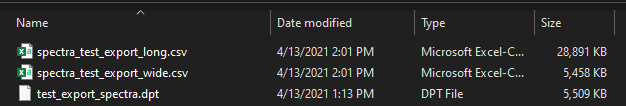
Reads a list object (as from read_dpt()). This function can be used to create outputs for MS excel users. It returns the following outputs: 1. Number of columns in the object 2. Number of particles where spectra are available 3. CSV in wide format 4. CSV in long format

The function spectra to long is integrated in this function.

spectra_to_csv(spectra = object_holding_spectra,
               out_path = r"(path\to\workspace)",
               out_file = "filename_for_csv")

Console Output example:

Nr of Columns in spectra file =  327
Nr of Particles in data =  326


 Renaming data...
done!


 Transform data to long format..
# A tibble: 630,484 x 3
   wavelength particle       absorbtion_unit
        <dbl> <chr>                    <dbl>
 1      3997. abs_particle1           -0.261
 2      3997. abs_particle2           -0.179
 3      3997. abs_particle3           -0.211
 4      3997. abs_particle4           -0.185
 5      3997. abs_particle5           -0.239
 6      3997. abs_particle6           -0.222
 7      3997. abs_particle7           -0.219
 8      3997. abs_particle8           -0.250
 9      3997. abs_particle9           -0.206
10      3997. abs_particle10          -0.218
# ... with 630,474 more rows
done!


 Write CSV long and wide format...
done!

Example

Choose particles and wavelength. Plot raw spectra.

spectra_to_long(spectra) -> spectra_dat

spectra_dat %>%
  filter(particle %in% c("abs_particle1", "abs_particle300"),
         wavelength > 1250 & wavelength < 3000) %>%
  ggplot(aes(x = wavelength, y = absorbtion_unit, color = particle, group = particle))+
  geom_line(show.legend = TRUE) +
  scale_x_reverse() 

toebR/OPUSdata documentation built on Feb. 14, 2022, 8:16 a.m.