inst/ws_desc/desc_3.13.md

In vjcitn/osca4anvil: Simplify production of computable OSCA texts and artifacts for AnVIL

We provide resources to compute with the Orchestrating Single Cell Analysis book. Use at least an 8 core machine to acquire packages and run workflows described in this workspace. More information on execution profiles (how much time and memory book-based jobs consume) is forthcoming.

About the book

The book has a few large sections:

• Introduction
• Basics
• Advanced tasks
• Workflows
• Multisample tasks

Each section has multiple chapters and code chunks that you will be able to evaluate in this workspace, once the package environment is properly set up. See Acquire all packages... below to accomplish this setup.

Many code chunks require certain antecedent computations to be completed before they will run. You may have to hunt back through preceding chunks to find the antecedents. If this proves impossible, please file a detailed bug report.

Taster

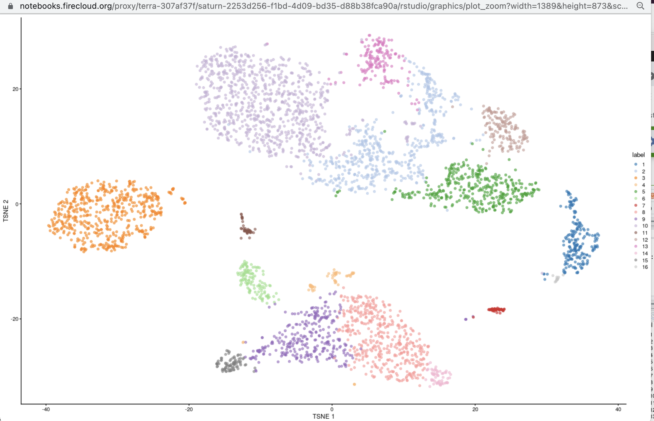
After following the setup instructions below, you can run the code snippet given towards the end of this description in Rstudio. In about 3 minutes, you will have acquired data on 4000 PBMCs published by TENxGenomics, performed basic QC and filtering, and computed projections and cluster assignments to yield

Starting out (Nov 7, 2021), using a Bioconductor 3.13 cloud environment:

Acquire helper package

BiocManager::install(c("AnVIL", "vjcitn/osca4anvil"), ask=FALSE)

library(osca4anvil)

Investigate the packages needed to run computations from OSCA book

The book is defined by five high-level R packages. The DESCRIPTION files of these packages define section-specific dependencies, and when these and their downstream dependencies are satisfied, we require hundreds of packages to be available.

show_packs()

This produces a hyperlinked table with 436 entries. Links point to landing pages at bioconductor.org or CRAN.

Examples of interest are the landing page for scRNAseq and the associated vignette, both specific to Bioconductor 3.13.

Acquire all packages needed to run computations from the book

Strictly speaking, the process defined below is not necessary. A reader can attempt a computation, and it may fail owing to the lack of a package. One can then use AnVIL::install to obtain the missing package. But this process may recur frequently. Thus we advocate the following steps to be taken, which will take some time to complete, but will provide all packages needed to perform any computational example in the book.

clone_osca()

lapply(packs(), get_deps, installer=AnVIL::install)  # Ncpus argument?

Example

Once we have installed all the packages using the code chunk just above, we can get the following example done in about 3 minutes. This is from OSCA.workflows demonstrating end-to-end analysis of 4000 unfiltered PBMCs.

# acquire data (caching if necessary) and create SingleCellExperiment

library(DropletTestFiles)
raw.path <- getTestFile("tenx-2.1.0-pbmc4k/1.0.0/raw.tar.gz")
out.path <- file.path(tempdir(), "pbmc4k")
untar(raw.path, exdir=out.path)

library(DropletUtils)
fname <- file.path(out.path, "raw_gene_bc_matrices/GRCh38")
sce.pbmc <- read10xCounts(fname, col.names=TRUE)

# identify cells with high abundance of mitochondrial genes

library(scater)
rownames(sce.pbmc) <- uniquifyFeatureNames(
  rowData(sce.pbmc)$ID, rowData(sce.pbmc)$Symbol)

library(EnsDb.Hsapiens.v86)
location <- mapIds(EnsDb.Hsapiens.v86, keys=rowData(sce.pbmc)$ID, 
                   column="SEQNAME", keytype="GENEID")

# perform cell detection

set.seed(100)
e.out <- emptyDrops(counts(sce.pbmc))
sce.pbmc <- sce.pbmc[,which(e.out$FDR <= 0.001)]

unfiltered <- sce.pbmc

# remove high-mito cells

stats <- perCellQCMetrics(sce.pbmc, subsets=list(Mito=which(location=="MT")))
high.mito <- isOutlier(stats$subsets_Mito_percent, type="higher")
sce.pbmc <- sce.pbmc[,!high.mito]

# normalize

library(scran)
set.seed(1000)
clusters <- quickCluster(sce.pbmc)
sce.pbmc <- computeSumFactors(sce.pbmc, cluster=clusters)
sce.pbmc <- logNormCounts(sce.pbmc)

# identify highly variable genes

set.seed(1001)
dec.pbmc <- modelGeneVarByPoisson(sce.pbmc)
top.pbmc <- getTopHVGs(dec.pbmc, prop=0.1)

# project; cluster

set.seed(10000)
sce.pbmc <- denoisePCA(sce.pbmc, subset.row=top.pbmc, technical=dec.pbmc)

set.seed(100000)
sce.pbmc <- runTSNE(sce.pbmc, dimred="PCA")

set.seed(1000000)
sce.pbmc <- runUMAP(sce.pbmc, dimred="PCA")

g <- buildSNNGraph(sce.pbmc, k=10, use.dimred = 'PCA')
clust <- igraph::cluster_walktrap(g)$membership
colLabels(sce.pbmc) <- factor(clust)

# visualize

plotTSNE(sce.pbmc, colour_by="label")

Execution profile

The following graphic illustrates the use of CPU, memory, disk, and network in the execution of the script given above on an 8 core, 30GB Terra instance.

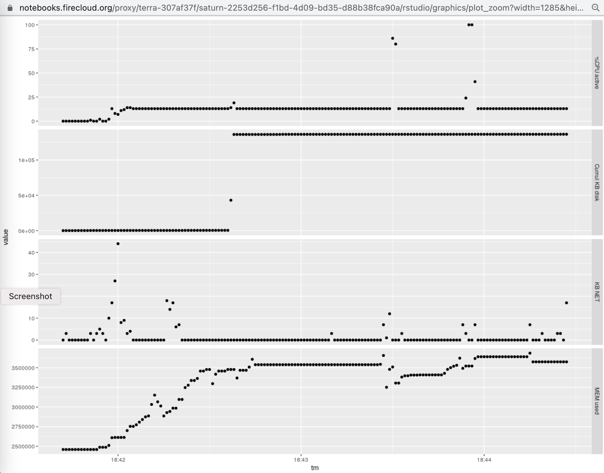
Of note is the total memory consumption of around 4GB (units are kilobytes), and the occurrence of short events in which the baseline CPU consumption rose from around 1/8 (one of 8 cores) to around 1 (all 8 cores mobilized). The analysis of RAM usage by the specific tasks undertaken involves subtracting the maximum from minimum displayed. This indicates that RAM usage over the baseline required by Rstudio and basic package loading never exceeded 1.5.GB.

vjcitn/osca4anvil documentation built on May 22, 2024, 10:23 a.m.