README.md

In vsbuffalo/msr: Call and parse MS from R

Call/Parse/Analyze Hudson's MS coalescent simulator results from R

This is a tiny package to call/parse MS results from R. I got sort of sick of saving MS output to file and loading it into R each time I wanted a quick graphic. The design is in following with Hadley's purrr and dplyr-driven tidy way of manipulating dataframes (or in this case, tibbles).

Example: Calculating Theta Pi and Watterson's Theta

Here's a simple example:

> library(msr)
> library(tidyverse)
> res <- call_ms(10, 100, t=5) %>% parse_ms() %>% 
            mutate(pi=map_dbl(gametes, theta_pi))
> res
# A tibble: 100 × 5
     rep segsites  positions         gametes    pi
   <int>    <dbl>     <list>          <list> <dbl>
1      1       19 <dbl [19]> <int [10 × 19]>  6.06
2      2       14 <dbl [14]> <int [10 × 14]>  3.64
3      3       21 <dbl [21]> <int [10 × 21]>  6.58
4      4       21 <dbl [21]> <int [10 × 21]>  6.20
5      5       12 <dbl [12]> <int [10 × 12]>  4.56
6      6        4  <dbl [4]>  <int [10 × 4]>  1.56
7      7       13 <dbl [13]> <int [10 × 13]>  4.10
8      8        9  <dbl [9]>  <int [10 × 9]>  2.62
9      9       16 <dbl [16]> <int [10 × 16]>  5.92
10    10       12 <dbl [12]> <int [10 × 12]>  3.32
# ... with 90 more rows

Note that call_ms() (and its sibling function ms(), which also automatically parses the results) take arguments in two ways: (1) as a command line string, and (2) as function arguments (as theta was specified above). For the latter, multiple-valued arguments are passed as a vector, e.g. to run ms with a theta of 30 (-t 30), a rho of 10 for 1000 sites (-r 10 1000), sampling 10 gametes, and replicated 100 times use: ms(10, 1000, t=30, r=c(10, 1000)). Taking arguments directly through the function like this makes calling MS with multiple parameters easier, through the purrr function invoke_rows() (see further below).

Returning to our example above, we can now analyze these results, using the packaged summary statistics functions theta_pi() and theta_W() on the data (though see below for an alternate way with the function sample_stats():

> res <-  res %>% mutate(theta_pi=map_dbl(gametes, theta_pi), 
                         theta_W=theta_W(segsites, 10))
> res 
# A tibble: 100 × 7
     rep segsites  positions         gametes        pi  theta_pi   theta_W
   <int>    <dbl>     <list>          <list>     <dbl>     <dbl>     <dbl>
1      1       21 <dbl [21]> <int [15 × 21]>  6.506667  6.506667  7.423201
2      2       14 <dbl [14]> <int [15 × 14]>  4.817778  4.817778  4.948801
3      3       11 <dbl [11]> <int [15 × 11]>  3.537778  3.537778  3.888343
4      4       12 <dbl [12]> <int [15 × 12]>  2.293333  2.293333  4.241829
5      5       24 <dbl [24]> <int [15 × 24]>  7.431111  7.431111  8.483658
6      6       44 <dbl [44]> <int [15 × 44]> 16.551111 16.551111 15.553374
7      7       20 <dbl [20]> <int [15 × 20]>  5.066667  5.066667  7.069715
8      8       15 <dbl [15]> <int [15 × 15]>  2.275556  2.275556  5.302286
9      9       18 <dbl [18]> <int [15 × 18]>  5.617778  5.617778  6.362744
10    10       19 <dbl [19]> <int [15 × 19]>  7.253333  7.253333  6.716229
# ... with 90 more rows

Now, we find the mean of these summary statistics:

> res %>% summarize(theta_pi = mean(theta_pi), theta_W = mean(theta_W))
 A tibble: 1 × 2
  theta_pi  theta_W
     <dbl>    <dbl>
1 4.950222 6.062281

The list-column approach stores the site matrices for each run in a gametes list-column. Each element of the list is a matrix. Similarly, positions is a list-column, where each element is a vector of positions. Calculations on the gamete site matrix can be done using the mutate(stat = map_dbl(gametes, some_fun)) dplyr/purrr pattern (see the example above).

Sample Statistics

Some basic sample statistics functions like those in MS's sample_stats package are included in the package: theta_W(), theta_pi(), tajd(), and a function sample_stats() that calculates these in a pipeline.

To make quick runs simple, ms() runs both call_ms() and parse_ms(). We combine this with sample_stats() below:

> ms(nsam=10, howmany=50, t=30) %>% sample_stats(.n=10) %>% 
    summarize(theta_pi = mean(theta_pi), theta_W = mean(theta_W))

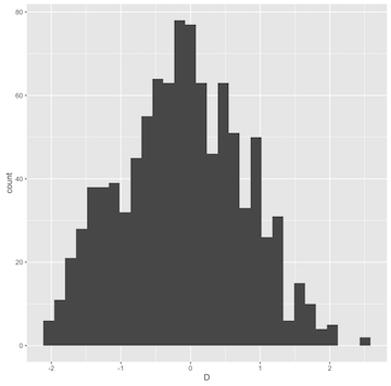
Or, a quick graphic example:

ggplot(ms(10, 1000, t=30) %>% sample_stats(.n=10)) + geom_histogram(aes(x=D))

Writing Output to File

It's likely for reproducibility's sake you'd like to save the MS run to file. You can do this, still sending the output to the pipe with write_tee():

> call_ms(10, 100, "-t 5") %>% write_tee("ms.out") %>%
   parse_ms() %>% mutate(pi=map_dbl(gametes, theta_pi))

# A tibble: 100 × 5
     rep segsites  positions         gametes    pi
   <int>    <dbl>     <list>          <list> <dbl>
1      1        8  <dbl [8]>  <int [10 × 8]>  1.86
2      2       13 <dbl [13]> <int [10 × 13]>  2.58
3      3        4  <dbl [4]>  <int [10 × 4]>  1.64
4      4       14 <dbl [14]> <int [10 × 14]>  3.86
5      5       20 <dbl [20]> <int [10 × 20]>  4.98
6      6        9  <dbl [9]>  <int [10 × 9]>  3.10
7      7        3  <dbl [3]>  <int [10 × 3]>  1.08
8      8       11 <dbl [11]> <int [10 × 11]>  3.10
9      9       23 <dbl [23]> <int [10 × 23]> 10.32
10    10       28 <dbl [28]> <int [10 × 28]> 10.02
# ... with 90 more rows

MS Runs Across Multiple Parameters

The purrr package has a really nice feature: if we have rows of a dataframe representing a set of parameters, we can "invoke" a function on these parameters with the function invoke_row() (or by_rows()). With msr, this is useful if you want to analyze the results of multiple MS runs across different parameter values. While this is possible with other approaches in R, it's much easier using the tidy data approach. Below, I replicate Table 1 of Kevin Thornton's neat paper Recombination and the Properties of Tajima's D in the Context of Approximate-Likelihood Calculation using this approach (though do note that I am using N=10^4 rather than N=10^5 as in the paper since our department's happy hour is soon, and I didn't want to wait for simulations to complete for this example):

> library(tidyverse)
> library(msr)

# generate the parameter tibble:
> params <- tibble(nsam=30, howmany=10^4, t=20, 
                  r=list(c(0, 1e3), c(10, 1e3), c(50, 1e3))) 

# run the simulations
> res <- params %>% invoke_rows(.f=ms, .to="msout")

# append a sample_stats list-column, calculating sample_stats on each MS run,
# then unnest, bringing these columns into the main tibble
> stats <- res %>% mutate(rho=map_dbl(r, first)) %>% 
              mutate(sample_stats=map(msout, sample_stats, .n=first(nsam))) %>% 
              unnest(sample_stats)

# group by all changing parameters, and calc summaries of the summary statistics
> stats %>% group_by(rho) %>% 
     mutate(D_num=tajd_num(theta_pi, segsites, first(nsam)), 
            D_denom=tajd_denom(segsites, first(nsam))) %>%
     summarize(ED=mean(D), E_D=mean(D_num)/mean(D_denom))
# A tibble: 3 × 3
    rho          ED           E_D
  <dbl>       <dbl>         <dbl>
1     0 -0.11336280 -0.0110814556
2    10 -0.04110813 -0.0025031942
3    50 -0.01035947 -0.0009970084

This table is reasonably close to Thornton's Table 1, showing the same trend downward trend (though there is a lot of variability across runs due to the smallish number of replicates).

Different Simulators

Many coalescent simulators can output data in MS-like format (e.g. Jerome Kelleher's awesome msprime). These can be used as executables too; just specify ms=mspms in the ms() or call_ms() functions. Note that no argument checking is done in this package; function arguments passed through ... are run through a simple set of rules to convert them to command line arguments, and then these are passed to the executable. Here's an example of using msprime's mspms command line program:

> ms(30, 100, t=20, ms="mspms") %>% sample_stats(.n=30)
# A tibble: 100 × 7
     rep segsites  positions         gametes  theta_pi   theta_W           D
   <int>    <dbl>     <list>          <list>     <dbl>     <dbl>       <dbl>
1      1       79 <dbl [79]> <int [30 × 79]> 23.696552 19.941167  0.71473150
2      2       83 <dbl [83]> <int [30 × 83]> 19.728736 20.950846 -0.22172280
3      3       88 <dbl [88]> <int [30 × 88]> 20.664368 22.212946 -0.26544457
4      4       88 <dbl [88]> <int [30 × 88]> 34.751724 22.212946  2.14929525
5      5       86 <dbl [86]> <int [30 × 86]> 19.386207 21.708106 -0.40698671
6      6       66 <dbl [66]> <int [30 × 66]> 15.434483 16.659709 -0.27739707
7      7       34 <dbl [34]> <int [30 × 34]>  8.278161  8.582274 -0.12919050
8      8       46 <dbl [46]> <int [30 × 46]> 10.554023 11.611312 -0.33800589
9      9       63 <dbl [63]> <int [30 × 63]> 16.025287 15.902450  0.02908369
10    10       96 <dbl [96]> <int [30 × 96]> 30.098851 24.232304  0.92399683
# ... with 90 more rows

Working with Trees

Using the option -T in MS outputs an additional entry: Newick-formatted trees. msr automatically detects this, and adds a tree column of character-vector Newick-format trees. Below is an example:

> res <- ms(30, 100, t=20, T=TRUE)
> res %>% select(tree)
# A tibble: 100 × 1
                                       tree
                                      <chr>
1  (((10:0.088,11:0.088):0.154,(23:0.163,((
2  (((6:0.018,18:0.018):0.330,((19:0.001,24
3  (((4:0.071,((24:0.006,25:0.006):0.045,((
4  (((((((3:0.003,8:0.003):0.025,(19:0.008,
5  (((10:0.002,24:0.002):0.077,(3:0.008,22:
6  ((((9:0.022,(22:0.020,(13:0.015,(17:0.00
7  ((13:0.215,((23:0.001,26:0.001):0.170,(4
8  (((22:0.123,(15:0.030,(3:0.020,(9:0.003,
9  (((7:0.009,(18:0.001,30:0.001):0.008):0.
10 ((24:0.191,((11:0.016,20:0.016):0.031,(4
# ... with 90 more rows

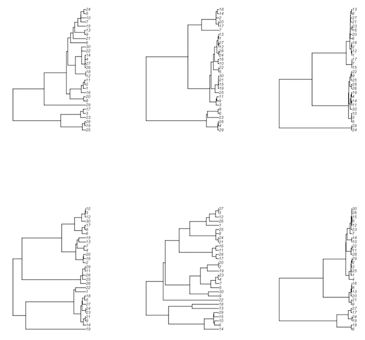
These can be plotted using a package like ape. Note that in the example there is no recombination, so there is one tree per simulation.

> library(ape)

# convert all trees using ape's read.tree()
> res <- ms(30, 100, t=20, T=TRUE)
> res <- res %>% mutate(ape_tree = read.tree(text=tree))

# store original par()
> opar <- par(no.readonly=TRUE)
> par(mfrow=c(2, 3))

# walk the sampled rows' tree objects (from ape), plotting each one
> res %>% sample_n(6) %>% mutate(x=walk(ape_tree, plot))

# restore par()
> par(opar)

With recombination, a single recombining locus's genealogy can no longer be described by a single tree. Consequently, the tree column is a list-column full of tibbles, each containing columns of the length of the segment (in bp) and the trees for each segment's marginal genealogy.

> res <- ms(30, 100, t=20, r=c(20, 100), T=TRUE)
> res <- res %>% sample_n(6) %>% 
           mutate(ape_tree=map(tree, ~read.tree(text=.$tree)))

Strict parsing

msr makes a guess about how to convert R's function arguments into flags for command line programs, based on the length of the flags (e.g. more than one character flags are automatically prefaced with --). This works with well-behaved command line programs like msprime, but fails with ms (e.g. with its -seeds flag). Use strict=TRUE and each . is converted to a -.

vsbuffalo/msr documentation built on May 3, 2019, 7:07 p.m.