README.md

In yanisb3812/DyrRegLog: Logistic Regression

DyrRegLog

Installing the package

To use the package, it has to be installed first.

devtools::install_github("yanisb3812/DyrRegLog")

Loading the library

When the package is installed, it can be loaded by using the library command from R.

library(DyrRegLog)

Dataset Import

A dataset is required to run the functions of this package. We'll be using the diabetes2 dataset.

data<-("diabetes2.csv")

Then we can use some commands from R to visualize our data.

str(data)

data.frame':    768 obs. of  9 variables:
 $ Pregnancies             : int  6 1 8 1 0 5 3 10 2 8 ...
 $ Glucose                 : int  148 85 183 89 137 116 78 115 197 125 ...
 $ BloodPressure           : int  72 66 64 66 40 74 50 0 70 96 ...
 $ SkinThickness           : int  35 29 0 23 35 0 32 0 45 0 ...
 $ Insulin                 : int  0 0 0 94 168 0 88 0 543 0 ...
 $ BMI                     : num  33.6 26.6 23.3 28.1 43.1 25.6 31 35.3 30.5 0 ...
 $ DiabetesPedigreeFunction: num  0.627 0.351 0.672 0.167 2.288 ...
 $ Age                     : int  50 31 32 21 33 30 26 29 53 54 ...
 $ Outcome                 : int  1 0 1 0 1 0 1 0 1 1 ...

 Now we can detect our target variable and we see that all the variables are numeric.
 It includes variables that can be the cause of the presence of diabetes, shown by the target variable "Outcome".


 summary(data)

  Pregnancies        Glucose      BloodPressure    SkinThickness      Insulin           BMI        DiabetesPedigreeFunction      Age           Outcome     
 Min.   : 0.000   Min.   :  0.0   Min.   :  0.00   Min.   : 0.00   Min.   :  0.0   Min.   : 0.00   Min.   :0.0780           Min.   :21.00   Min.   :0.000  
 1st Qu.: 1.000   1st Qu.: 99.0   1st Qu.: 62.00   1st Qu.: 0.00   1st Qu.:  0.0   1st Qu.:27.30   1st Qu.:0.2437           1st Qu.:24.00   1st Qu.:0.000  
 Median : 3.000   Median :117.0   Median : 72.00   Median :23.00   Median : 30.5   Median :32.00   Median :0.3725           Median :29.00   Median :0.000  
 Mean   : 3.845   Mean   :120.9   Mean   : 69.11   Mean   :20.54   Mean   : 79.8   Mean   :31.99   Mean   :0.4719           Mean   :33.24   Mean   :0.349  
 3rd Qu.: 6.000   3rd Qu.:140.2   3rd Qu.: 80.00   3rd Qu.:32.00   3rd Qu.:127.2   3rd Qu.:36.60   3rd Qu.:0.6262           3rd Qu.:41.00   3rd Qu.:1.000  
 Max.   :17.000   Max.   :199.0   Max.   :122.00   Max.   :99.00   Max.   :846.0   Max.   :67.10   Max.   :2.4200           Max.   :81.00   Max.   :1.000

 We can see that our variables are not on the same scale, we'll resolve that later on.
 ```
 After that, we'll define a size of sample.

 ```
 smp_size <- floor(0.70 * nrow(data))
 ```
 Here, we selected 70% of the data size.

 Then, we divide our sample into a training data and a test data randomly.

 ```
 set.seed(29112021)
 train_ind <- sample(seq_len(nrow(data)), size = smp_size)

 data_train <- data[train_ind, ]
 data_test <- data[-train_ind, ]
 ```

Now we can call the fit function of DyrRegLog package to fit our model to a Logistic Regression using the stochastic gradient descent algorithm.

test_fit = fit(formula = Outcome~. , data = data , eta = 0.3 , iter_Max = 10000 , mode = "Batch_Simple" , batch_size = 20, nb_Coeurs = 1 )

We can also visualize the plot of the deviances.
![image](https://user-images.githubusercontent.com/72911055/143915963-6803e291-85b4-4ef8-a339-8e311ca79d3d.png)


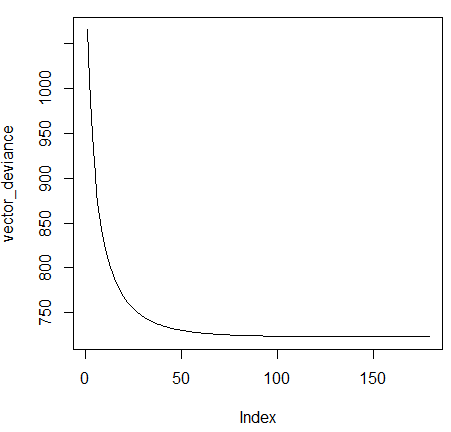
The print and summary functions are overridden.
So, if we print the variable containing the fit function, it will display the formula and the coefficients.

print(test_fit)

Formula : ~ Outcome .

Coefficients : Pregnancies Glucose BloodPressure SkinThickness Insulin BMI DiabetesPedigreeFunction Age Intercept 1 0.4080121 1.110398 -0.2523509 0.005541574 -0.1286005 0.7017453 0.3108529 0.1803396 -0.8660777

It is the same thing for the summary function, but it will display the last value of 
the deviance, the number of tierations and the time of execution of the algorithm.

summary(test_fit)

Last deviance value : 723.4693

Number of iterations : 180

Computing time : 0.35

Then we can predict our target variable with the predict function.

test_predict=predict(data_test[,-9], test_fit,sortie="Class") print(test_predict) [1] 0 1 0 0 1 0 1 1 1 1 1 1 1 1 1 1 1 1 0 1 1 0 1 1 0 1 0 1 0 1 1 1 0 1 0 0 1 [38] 1 0 1 0 1 0 1 0 1 1 0 0 1 1 1 1 1 0 1 1 1 1 0 1 1 1 1 1 0 1 1 0 1 1 1 1 1 [75] 1 1 0 0 1 1 0 0 1 1 1 1 1 0 1 1 1 0 1 1 1 1 1 0 1 1 1 1 1 1 1 1 1 1 0 1 1 [112] 1 1 1 1 1 1 0 0 1 0 1 1 1 0 1 1 1 1 1 0 1 1 0 0 1 1 1 1 0 1 1 0 0 1 1 1 0 [149] 1 1 1 1 0 0 0 0 1 1 1 1 1 1 0 1 1 0 1 1 1 1 1 0 1 1 1 1 0 1 1 1 0 1 0 0 1 [186] 1 1 1 0 0 1 1 1 0 1 1 0 1 0 0 1 1 1 1 1 1 1 1 1 0 0 1 1 1 0 0 1 0 1 0 1 1 [223] 0 1 0 1 1 1 1 1 1

We can evaluate the model using functions from the carret package.

library(caret) test_val=data_test[9] test_val=as.vector(test_val)

print(caret::confusionMatrix(as.factor(t(data_test[,9])),as.factor(test_predict))) Confusion Matrix and Statistics

      Reference

Prediction 0 1 0 63 87 1 3 78

           Accuracy : 0.6104          
             95% CI : (0.5442, 0.6737)
No Information Rate : 0.7143          
P-Value [Acc > NIR] : 0.9997

              Kappa : 0.3092

Mcnemar's Test P-Value : <2e-16

        Sensitivity : 0.9545          
        Specificity : 0.4727          
     Pos Pred Value : 0.4200          
     Neg Pred Value : 0.9630          
         Prevalence : 0.2857          
     Detection Rate : 0.2727

Detection Prevalence : 0.6494 Balanced Accuracy : 0.7136

   'Positive' Class : 0

```

You've completed the tutorial of the package functions. Thank you for doing so !

yanisb3812/DyrRegLog documentation built on Dec. 23, 2021, 7:15 p.m.