In yijunyang/bis557: BIS557 HW#1

knitr::opts_chunk$set(
  collapse = TRUE,
  comment = "#>"
)

library(bis557)
library(ggplot2)
library(caret)
library(gridExtra)

1 Introduction

Spirals are found in several natural domains, such as galaxies, shells, and double-helix DNA. Spiral structures are one of the most difficult patterns to classify because of their high levels of nonlinearity.

The two-spiral classification task for artificial neural networks was first proposed in the late 1980s by Lang and Whitbrock. Nowadays, there are several different packages available for this kind of classification task, but it is still important to understand the underlying logic of neural networks.

This project will be aimed at building a three-layer deep neural network and showing how to use neural networks for multi-classification. In addition, we will penalize the weights in the deep learning model and comparing the results with different choices of $\lambda$, to show how regularization solves the problem of overfitting.

2 Methods

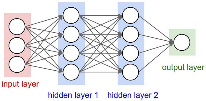
Neural networks are an extension of the linear approaches applied to the problem of detecting non-linear interactions in high-dimensional data. Neural networks consist of a collection of objects, known as neurons, organized into an ordered set of layers. The picture below shows a 3-layer neural network.

Back propagation

Training a neural network involves updating the parameters describing the connections in order to minimize some loss function over the training data. In the case of back propagation, the neural network first carries out a forward propagation, evaluates the loss of the model as per some defined cost function, adjusts the weights between the hidden layers accordingly, carries out another forward propagation, and so on and so forth for some defined number of iterations.

Activation function

The use of activation functions is essential to the functioning of neural networks. Activation functions are mathematical functions that allow neural networks to account for non-linear relationships. One of the popular choices is known as a rectified linear unit (ReLU), which pushes negative values to 0 while returns positive values unmodified:

$$ ReLU(x) = \left{ \begin{aligned} &x, \quad \text{if } x \ge 0\ &0, \quad \text{otherwise} \end{aligned} \right. $$

For classification tasks, we can convert a vector $y$ of integer coded classes into a matrix $Y$ containing indicator variables for each class. Treating the output layer as probabilities raise the concern that these values may not sum to 1 and could produce negative values or values greater than one depending on the inputs. Therefore, we need to apply a function to the output layer to make it behave like a proper set of probabilities. The activation we use is called the softmax function, defined as:

$$ softmax(z_j^L) = \frac{e^{z_j}}{\sum_k e^{z_j}} $$

In the 3-layer neural network, ReLU will be used as activation function for the first 2 layers (hidden layers). softmax will be used for the last layer since we need to make the output layer behave as a proper set of probabilities.

Loss function

Regularization by adding a penalty term to the loss function will be employed intended to penalize the weights and address overfitting. Here, we choose to add an $\ell_2$-norm as was done with ridge regression. The loss function is:

$$ \mathcal{L}=- \frac{1}{n} \sum_{i=1}^n log \; p(y=y_i|X_i)+ \frac{\lambda}{2}(\Vert W_1 \Vert _2^2 + \Vert W_2 \Vert _2^2 + \Vert W_3 \Vert _2^2) $$

Application

To prove the effectivness of our model, a simulated spiral data will be used for classification. The input $X \in \mathbb{R} ^{N\times2}$ will be 2-dimension. The response will be $y \in \mathbb{R} ^{N}$, which is the category indicator. The following plot visualize the dataset.

# print the spiral data
source("spiral_simulation.R")
print(source("spiral_simulation.R")$value)

3 Results

Math Derivation

From the above description, we construct a neural network model as below:

$$ h_1=ReLU(W_1X+b_1) \ h_2=ReLU(W_2h_1+b_2) \ p=softmax(W_3h_2+b_3) $$

where $h_1$ represents the results of the first hidden layer; $h_2$ represents the results of the second hidden layer; $p$ represents the results of the output layer, which is a matrix of probability. $W_1, W_2, W_3$ and $b_1, b_2, b_3$ are the weights and biases for the corresponding layer.

Then, we need to get the formulas for the derivatives for each layer of the network:

$$ \begin{aligned} \frac{\partial \mathcal{L}}{\partial W_3} &= \frac{1}{N}h_2^T(P-Y) + \lambda W_3 \ \frac{\partial \mathcal{L}}{\partial b_3} &= \left(\begin{array} {c} \frac{1}{N} \ \vdots \ \frac{1}{N} \end{array}\right) (P-Y) \ \ \frac{\partial \mathcal{L}}{\partial W_2} &= \frac{1}{N} h_1^T (P-Y) W_3^T\ \mathbf 1{h_2 > 0} + \lambda W_2 \ \frac{\partial \mathcal{L}}{\partial b_2} &= \left(\begin{array} {c} \frac{1}{N} \ \vdots \ \frac{1}{N} \end{array}\right) (P-Y) W_3^T\ \mathbf 1{h_2 > 0} \ \ \frac{\partial \mathcal{L}}{\partial W_1} &= \frac{1}{N} X^T (P-Y) W_3^T\ \mathbf 1{h_2 > 0} W_2^T\ \mathbf 1{h_1 > 0} + \lambda W_1 \ \frac{\partial \mathcal{L}}{\partial b_1} &= \left(\begin{array} {c} \frac{1}{N} \ \vdots \ \frac{1}{N} \end{array}\right) (P-Y) W_3^T\ \mathbf 1{h_2 > 0} W_2^T\ \mathbf 1{h_1 > 0} \end{aligned} $$

Coding Implementation

Coding are implemented with R version 4.0.3. All the relavent resources are introduced in Appendix.

In each hidden layer, there are 100 nodes.

model1 <- bis557::NN_classify(X, y, 
                      maxit = 1500, gamma = 0.1,
                      H1 =100, H2 = 100, lambda = 0)

model2 <- bis557::NN_classify(X, y, 
                      maxit = 1500, gamma = 0.1,
                      H1 =100, H2 = 100, lambda = 0.005)

model3 <- bis557::NN_classify(X, y, 
                      maxit = 1500, gamma = 0.1,
                      H1 =100, H2 = 100, lambda = 0.01)

model4 <- bis557::NN_classify(X, y, 
                      maxit = 1500, gamma = 0.1,
                      H1 =100, H2 = 100, lambda = 0.1)

par(mfrow=c(2,2))
prediction_result1 <- bis557::NN_pred(X, model1)
prediction_result2 <- bis557::NN_pred(X, model2)
prediction_result3 <- bis557::NN_pred(X, model3)
prediction_result4 <- bis557::NN_pred(X, model4)

bis557::plot_boundary(X, y, model1, "lambda = 0")
bis557::plot_boundary(X, y, model2, "lambda = 0.005")
bis557::plot_boundary(X, y, model3, "lambda = 0.01")
bis557::plot_boundary(X, y, model4, "lambda = 0.1")

# grid.arrange(p1, p2, p3, p4, ncol = 2)

mean(prediction_result1 == y)
mean(prediction_result2 == y)
mean(prediction_result3 == y)
mean(prediction_result4 == y)

Reference

[1] Arnold, T., Kane, M., & Lewis, B. W. (2019). A computational approach to statistical learning. CRC Press.

[2] A Neural Network Playground

[3] Build your own neural network classifier in R

[4] Coding Neural Network — Forward Propagation and Backpropagtion

[5] Explain the softmax function and related derivation process in detail

[6] Phyllotaxis - Draw flowers using mathematics

[7] Stephan K. Chalup & Lukasz Wiklendt (2007) Variations of the two-spiral task, Connection Science, 19:2, 183-199

[8] Understanding Regularization in Logistic Regression

yijunyang/bis557 documentation built on Dec. 21, 2020, 3:06 a.m.