README.md
In yufree/mzrtsim: Raw data (mzML) and peaks list simulation for LC/GC-MS based metabolomics data
mzrtsim


The goal of mzrtsim is to make raw data and features table simulation
for LC/GC-MS based data
Installation
You can install the development version from
GitHub with:
# install.packages("remotes")
remotes::install_github("yufree/mzrtsim")
Raw Data simulation
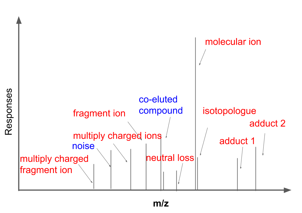
MS1 full scan data has been proved more complex than theoretical
prediction. Recently study showed that soft ionization will also contain
fragment ions for
structure identification and contain lots of redundant
peaks. As shown
in the following figure, MS1 full scan data could contain different
types of ions from the same compound (red). Some peaks we could figure
out the sources while some peaks might be hard to interpret. In this
case, mzrtsim package will use experimental data instead of predicted
peaks from the compound formula to show the complexity of MS1 spectra.
 demo
demo
You could use simmzml to generate one mzML file.
library(mzrtsim)
data("monams1")
simmzml(db=monams1, name = 'test')
You will find test.mzML and corresponding test.csv with m/z,
retention time and compound name of the peaks. Here the monams1 and
monahrms1 is from the MS1 data of MassBank of North America (MoNA) and
could be downloaded from their
website. You could also
use hmdbcms to simulate EI source data extracted from
HMDB. Here we only use the MS1 full scan
data for simulation.
Data extraction
For HMDB, you need to download their “GC-MS Spectra Files (XML) -
Experimental” data here. Then you need the
following R code to construct the database for this package.
xmlpath <- list.files('hmdb_experimental_cms_spectra/',full.names = T,recursive = T)
library(xml2)
getcms <- function(i){
  tree = xml2::read_xml(xmlpath[i])
  accession = xml_text(xml2::xml_find_all(tree,'/c-ms/database-id'))
  rti = as.numeric(xml_text(xml2::xml_find_all(tree,'/c-ms/retention-index')))
  prec = as.numeric(xml_text(xml2::xml_find_all(tree,'/c-ms/derivative-exact-mass')))
  formula = xml_text(xml2::xml_find_all(tree,'/c-ms/derivative-formula'))
  ins = xml_text(xml2::xml_find_all(tree,'/c-ms/notes'))
  ins2 = xml_text(xml2::xml_find_all(tree,'/c-ms/instrument-type'))
  mode = xml_text(xml2::xml_find_all(tree,'/c-ms/ionization-mode'))
  idms = xml_text(xml2::xml_find_all(tree,'/c-ms/id'))
  instr = xml_text(xml2::xml_find_all(tree,'instrument-type'))
  masscharge = as.numeric(xml_text(xml2::xml_find_all(tree,'/c-ms/c-ms-peaks/c-ms-peak/mass-charge')))
  intensity =  as.numeric(xml_text(xml2::xml_find_all(tree,'/c-ms/c-ms-peaks/c-ms-peak/intensity')))
  idx <- intensity!=0
  mz <- list(name=accession, idms=idms, ionmode=mode, prec = prec, formula = formula, np = length(masscharge[idx]), rti = rti, instr = ins2, msm = ins, spectra=cbind.data.frame(mz=masscharge[idx],ins=intensity[idx]))
  return(mz)
}

library(parallel)
hmdbcms <- mcMap(getcms,1:length(xmlpath), mc.cores = 4)
saveRDS(hmdbcms,'hmdbcms.RDS')
For MoNA, you can download the “LC-MS Spectra” data in format of “msp”
from this website. Then
we need to filter the MS1 data to generate database for LC-MS and subset
data base for LC-HRMS.
# you need to install enviGCMS package by 'install.packages("enviGCMS")'.
msp <- enviGCMS::getMSP('MoNA-export-LC-MS_Spectra.msp')
idx <- sapply(msp, function(x) grepl('MS1',x$msm))
idx1 <- sapply(idx, function(x) length(x)>0)
monams1 <- msp[idx1]
idx2 <- sapply(monams1, function(x) grepl('MS1',x$msm))
monams1 <- monams1[idx2]

idx3 <- sapply(monams1, function(x) x$instr )
idx4 <- sapply(idx3, function(x) length(x)>0)
monams12 <- monams1[idx4]
saveRDS(monams12,'monams1.RDS')

idx5 <- sapply(monams12, function(x) x$instr )
monams13 <- monams12[grepl('FT|TOF',idx5)]
idx5 <- sapply(monams13, function(x) x$instr )

nn <- sapply(monams13,function(x) x$np)
median(as.numeric(nn))
mean(as.numeric(nn))
saveRDS(monams13,'monahrms1.RDS')
If you have your own database in “msp” format, you can generate the
custom database by the following code:
msp <- enviGCMS::getMSP('MoNA-export-LC-MS_Spectra.msp')
saveRDS(msp,'custom.RDS')
To use the “*.RDS” database, you need to load them and refer their name
for ‘simmzml’ function.
custom <- readRDS('custom.RDS')
simmzml(db=custom, name = 'test')
Multiple files with experiment design
You could stimulate two groups of raw data with different peak heights
for the same compounds. Retention time will follow a uniform
distribution. 100 compounds could be selected randomly and base peaks’
signal to noise ratio could be sampled from 100 to 1000. When signal to
noise ratio is fixed for all samples, the peaks height will still be the
only changed parameters for both groups. Each group contain 10 samples
and 30% compounds are changed between case and control groups.
dir.create('case')
dir.create('control')
# set different peak width for 100 compounds
ph1 <- c(rep(5,30),rep(10,40),rep(15,30))
ph2 <- c(rep(5,20),rep(10,30),rep(15,50))
# set retention time for 100 compounds. When the peak width is set as a single value, the simulated base peak width will be from a poisson distribution with this value as lambda.
rt <- seq(10,590,length.out=100)
set.seed(1)
# select compounds from database
compound <- sample(c(1:4000),100)
set.seed(2)
# select signal to noise ratio for a larger dynamic range
sn <- sample(c(100:10000),100)
for(i in c(1:10)){
  simmzml(name=paste0('case/case',i),db=monahrms1,pheight = ph1,compound=compound,rtime = rt, sn=sn)
}

for(i in c(1:10)){
  simmzml(name=paste0('control/control',i),db=monahrms1,pheight = ph2,compound=compound,rtime = rt, sn=sn)
}
Then you could find 10 mzML files in case sub folder and another 10 mzML
files in control sub folder, as well as corresponding csv files with
m/z, retention time and compound name of the peaks.
If you prefer to simulate retention time shifts for different samples,
you could add a random number to the retention time of each compound.
rt0 <- rt
set.seed(42)
for(i in c(1:10)){
        rt <- rt0 + rnorm(100)
        simmzml(name=paste0('case/case',i),db=monahrms1,pwidth = pw1,compound=compound,rtime = rt, sn=sn)
}
Chromatography peaks
You could also use simmzml to stimulate tailing/leading peaks by
defining the tailing factor of the peaks. When the tailing factor is
lower than 1, the peaks are leading peaks. When the tailing factor is
larger than 1, the peaks are tailing peaks.
# leading peaks
simmzml(name='test',db=monahrms1,pwidth = 10,compound=1,rtime = 100, sn=10,tailingfactor = 0.8)
# tailing peaks
simmzml(name='test',db=monahrms1,pwidth = 10,compound=1,rtime = 100, sn=10,tailingfactor = 1.5)
matrix stimulation
You could also input a m/z vector as matrix masses. Those masses will
generate background baseline signals. By default, the mass vector is
from matrix samples previous
published.
data(mzm)
simmzml(name='test',db=monahrms1,pwidth = 10,compound=1,rtime = 100, sn=10,matrixmz = mzm,matrix = TRUE)
Peaks list simulation
You could also use mzrtsim to make simulation of peak list.
Here we make a simulation of 100 compounds from selected database with
two conditions and three batches. 5 percentage of the peaks were
influenced by conditions and 10 percentage of the peaks were influenced
by batch effects. Three different type could be simulated: monotonic,
random and block. You could also bind batch type, for example, ‘mb’
means the simulation would contain both monotonic and block batch
effects. ‘db’ means the spectra database to be used for simulation as
metioned in raw data simulation section.
library(mzrtsim)
data("monams1")
simdata <- mzrtsim(ncomp = 100, ncond = 2, ncpeaks = 0.05,
  nbatch = 3, nbpeaks = 0.1, npercond = 10, nperbatch = c(8, 5, 7), seed = 42, batchtype = 'mb', db=monams1)
You could save the simulated data into multiple csv files by simdata
function. simraw.csv could be used for metaboanalyst. simraw2.csv
show the raw peaks list. simcon.csv show peaks influenced by
conditions only.simbatchmatrix.csv show peaks influnced by batch
effects only. simbat.csv show peaks influenced by batch effects and
conditions. simcomp.csv show independent peaks influenced by
conditions and batch effects. simcompchange.csv show the conditions
changes of each groups. simblockbatchange.csv show the block batch
changes of each groups. simmonobatchange.csv show the monotonic batch
changes of each group.
simdata(sim,name = "sim")
yufree/mzrtsim documentation built on Feb. 18, 2025, 6:29 a.m.
R Package Documentation
Browse R Packages
We want your feedback!
Note that we can't provide technical support on individual packages. You should contact the package authors for that.
mzrtsim
![]()
![]()
The goal of mzrtsim is to make raw data and features table simulation for LC/GC-MS based data
Installation
You can install the development version from GitHub with:
# install.packages("remotes")
remotes::install_github("yufree/mzrtsim")
Raw Data simulation
MS1 full scan data has been proved more complex than theoretical prediction. Recently study showed that soft ionization will also contain fragment ions for structure identification and contain lots of redundant peaks. As shown in the following figure, MS1 full scan data could contain different types of ions from the same compound (red). Some peaks we could figure out the sources while some peaks might be hard to interpret. In this case, mzrtsim package will use experimental data instead of predicted peaks from the compound formula to show the complexity of MS1 spectra.
demo
You could use simmzml to generate one mzML file.
library(mzrtsim)
data("monams1")
simmzml(db=monams1, name = 'test')
You will find test.mzML and corresponding test.csv with m/z,
retention time and compound name of the peaks. Here the monams1 and
monahrms1 is from the MS1 data of MassBank of North America (MoNA) and
could be downloaded from their
website. You could also
use hmdbcms to simulate EI source data extracted from
HMDB. Here we only use the MS1 full scan
data for simulation.
Data extraction
For HMDB, you need to download their “GC-MS Spectra Files (XML) - Experimental” data here. Then you need the following R code to construct the database for this package.
xmlpath <- list.files('hmdb_experimental_cms_spectra/',full.names = T,recursive = T)
library(xml2)
getcms <- function(i){
tree = xml2::read_xml(xmlpath[i])
accession = xml_text(xml2::xml_find_all(tree,'/c-ms/database-id'))
rti = as.numeric(xml_text(xml2::xml_find_all(tree,'/c-ms/retention-index')))
prec = as.numeric(xml_text(xml2::xml_find_all(tree,'/c-ms/derivative-exact-mass')))
formula = xml_text(xml2::xml_find_all(tree,'/c-ms/derivative-formula'))
ins = xml_text(xml2::xml_find_all(tree,'/c-ms/notes'))
ins2 = xml_text(xml2::xml_find_all(tree,'/c-ms/instrument-type'))
mode = xml_text(xml2::xml_find_all(tree,'/c-ms/ionization-mode'))
idms = xml_text(xml2::xml_find_all(tree,'/c-ms/id'))
instr = xml_text(xml2::xml_find_all(tree,'instrument-type'))
masscharge = as.numeric(xml_text(xml2::xml_find_all(tree,'/c-ms/c-ms-peaks/c-ms-peak/mass-charge')))
intensity = as.numeric(xml_text(xml2::xml_find_all(tree,'/c-ms/c-ms-peaks/c-ms-peak/intensity')))
idx <- intensity!=0
mz <- list(name=accession, idms=idms, ionmode=mode, prec = prec, formula = formula, np = length(masscharge[idx]), rti = rti, instr = ins2, msm = ins, spectra=cbind.data.frame(mz=masscharge[idx],ins=intensity[idx]))
return(mz)
}
library(parallel)
hmdbcms <- mcMap(getcms,1:length(xmlpath), mc.cores = 4)
saveRDS(hmdbcms,'hmdbcms.RDS')
For MoNA, you can download the “LC-MS Spectra” data in format of “msp” from this website. Then we need to filter the MS1 data to generate database for LC-MS and subset data base for LC-HRMS.
# you need to install enviGCMS package by 'install.packages("enviGCMS")'.
msp <- enviGCMS::getMSP('MoNA-export-LC-MS_Spectra.msp')
idx <- sapply(msp, function(x) grepl('MS1',x$msm))
idx1 <- sapply(idx, function(x) length(x)>0)
monams1 <- msp[idx1]
idx2 <- sapply(monams1, function(x) grepl('MS1',x$msm))
monams1 <- monams1[idx2]
idx3 <- sapply(monams1, function(x) x$instr )
idx4 <- sapply(idx3, function(x) length(x)>0)
monams12 <- monams1[idx4]
saveRDS(monams12,'monams1.RDS')
idx5 <- sapply(monams12, function(x) x$instr )
monams13 <- monams12[grepl('FT|TOF',idx5)]
idx5 <- sapply(monams13, function(x) x$instr )
nn <- sapply(monams13,function(x) x$np)
median(as.numeric(nn))
mean(as.numeric(nn))
saveRDS(monams13,'monahrms1.RDS')
If you have your own database in “msp” format, you can generate the custom database by the following code:
msp <- enviGCMS::getMSP('MoNA-export-LC-MS_Spectra.msp')
saveRDS(msp,'custom.RDS')
To use the “*.RDS” database, you need to load them and refer their name for ‘simmzml’ function.
custom <- readRDS('custom.RDS')
simmzml(db=custom, name = 'test')
Multiple files with experiment design
You could stimulate two groups of raw data with different peak heights for the same compounds. Retention time will follow a uniform distribution. 100 compounds could be selected randomly and base peaks’ signal to noise ratio could be sampled from 100 to 1000. When signal to noise ratio is fixed for all samples, the peaks height will still be the only changed parameters for both groups. Each group contain 10 samples and 30% compounds are changed between case and control groups.
dir.create('case')
dir.create('control')
# set different peak width for 100 compounds
ph1 <- c(rep(5,30),rep(10,40),rep(15,30))
ph2 <- c(rep(5,20),rep(10,30),rep(15,50))
# set retention time for 100 compounds. When the peak width is set as a single value, the simulated base peak width will be from a poisson distribution with this value as lambda.
rt <- seq(10,590,length.out=100)
set.seed(1)
# select compounds from database
compound <- sample(c(1:4000),100)
set.seed(2)
# select signal to noise ratio for a larger dynamic range
sn <- sample(c(100:10000),100)
for(i in c(1:10)){
simmzml(name=paste0('case/case',i),db=monahrms1,pheight = ph1,compound=compound,rtime = rt, sn=sn)
}
for(i in c(1:10)){
simmzml(name=paste0('control/control',i),db=monahrms1,pheight = ph2,compound=compound,rtime = rt, sn=sn)
}
Then you could find 10 mzML files in case sub folder and another 10 mzML files in control sub folder, as well as corresponding csv files with m/z, retention time and compound name of the peaks.
If you prefer to simulate retention time shifts for different samples, you could add a random number to the retention time of each compound.
rt0 <- rt
set.seed(42)
for(i in c(1:10)){
rt <- rt0 + rnorm(100)
simmzml(name=paste0('case/case',i),db=monahrms1,pwidth = pw1,compound=compound,rtime = rt, sn=sn)
}
Chromatography peaks
You could also use simmzml to stimulate tailing/leading peaks by
defining the tailing factor of the peaks. When the tailing factor is
lower than 1, the peaks are leading peaks. When the tailing factor is
larger than 1, the peaks are tailing peaks.
# leading peaks
simmzml(name='test',db=monahrms1,pwidth = 10,compound=1,rtime = 100, sn=10,tailingfactor = 0.8)
# tailing peaks
simmzml(name='test',db=monahrms1,pwidth = 10,compound=1,rtime = 100, sn=10,tailingfactor = 1.5)
matrix stimulation
You could also input a m/z vector as matrix masses. Those masses will generate background baseline signals. By default, the mass vector is from matrix samples previous published.
data(mzm)
simmzml(name='test',db=monahrms1,pwidth = 10,compound=1,rtime = 100, sn=10,matrixmz = mzm,matrix = TRUE)
Peaks list simulation
You could also use mzrtsim to make simulation of peak list.
Here we make a simulation of 100 compounds from selected database with two conditions and three batches. 5 percentage of the peaks were influenced by conditions and 10 percentage of the peaks were influenced by batch effects. Three different type could be simulated: monotonic, random and block. You could also bind batch type, for example, ‘mb’ means the simulation would contain both monotonic and block batch effects. ‘db’ means the spectra database to be used for simulation as metioned in raw data simulation section.
library(mzrtsim)
data("monams1")
simdata <- mzrtsim(ncomp = 100, ncond = 2, ncpeaks = 0.05,
nbatch = 3, nbpeaks = 0.1, npercond = 10, nperbatch = c(8, 5, 7), seed = 42, batchtype = 'mb', db=monams1)
You could save the simulated data into multiple csv files by simdata
function. simraw.csv could be used for metaboanalyst. simraw2.csv
show the raw peaks list. simcon.csv show peaks influenced by
conditions only.simbatchmatrix.csv show peaks influnced by batch
effects only. simbat.csv show peaks influenced by batch effects and
conditions. simcomp.csv show independent peaks influenced by
conditions and batch effects. simcompchange.csv show the conditions
changes of each groups. simblockbatchange.csv show the block batch
changes of each groups. simmonobatchange.csv show the monotonic batch
changes of each group.
simdata(sim,name = "sim")
R Package Documentation
Browse R Packages
We want your feedback!
Note that we can't provide technical support on individual packages. You should contact the package authors for that.
Embedding an R snippet on your website
Add the following code to your website.
For more information on customizing the embed code, read Embedding Snippets.