README.md

In cola: A Framework for Consensus Partitioning

cola: A General Framework for Consensus Partitioning

Features

1. It modularizes the consensus clustering processes that various methods can be easily integrated in different steps of the analysis.
2. It provides rich visualizations for intepreting the results.
3. It allows running multiple methods at the same time and provides functionalities to compare results in a straightforward way.
4. It provides a new method to extract features which are more efficient to separate subgroups.
5. It generates detailed HTML reports for the complete analysis.

Install

cola is available on Bioconductor, you can install it by:

if (!requireNamespace("BiocManager", quietly = TRUE))
    install.packages("BiocManager")
BiocManager::install("cola")

The latest version can be installed directly from GitHub:

library(devtools)
install_github("jokergoo/cola")

Links

Examples for cola analysis can be found at https://jokergoo.github.io/cola_examples/ and https://jokergoo.github.io/cola_collection/.

Online documentation is at https://jokergoo.github.io/cola.

Supplementary for the cola manuscript is at https://github.com/jokergoo/cola_supplementary and the scripts are at https://github.com/jokergoo/cola_manuscript.

Vignettes

1. A Quick Start of Using cola Package
2. A Framework for Consensus Partitioning
3. Automatic Functional Enrichment on Signature genes
4. Predict Classes for New Samples
5. Work with Big Datasets

Consensus Partitioning

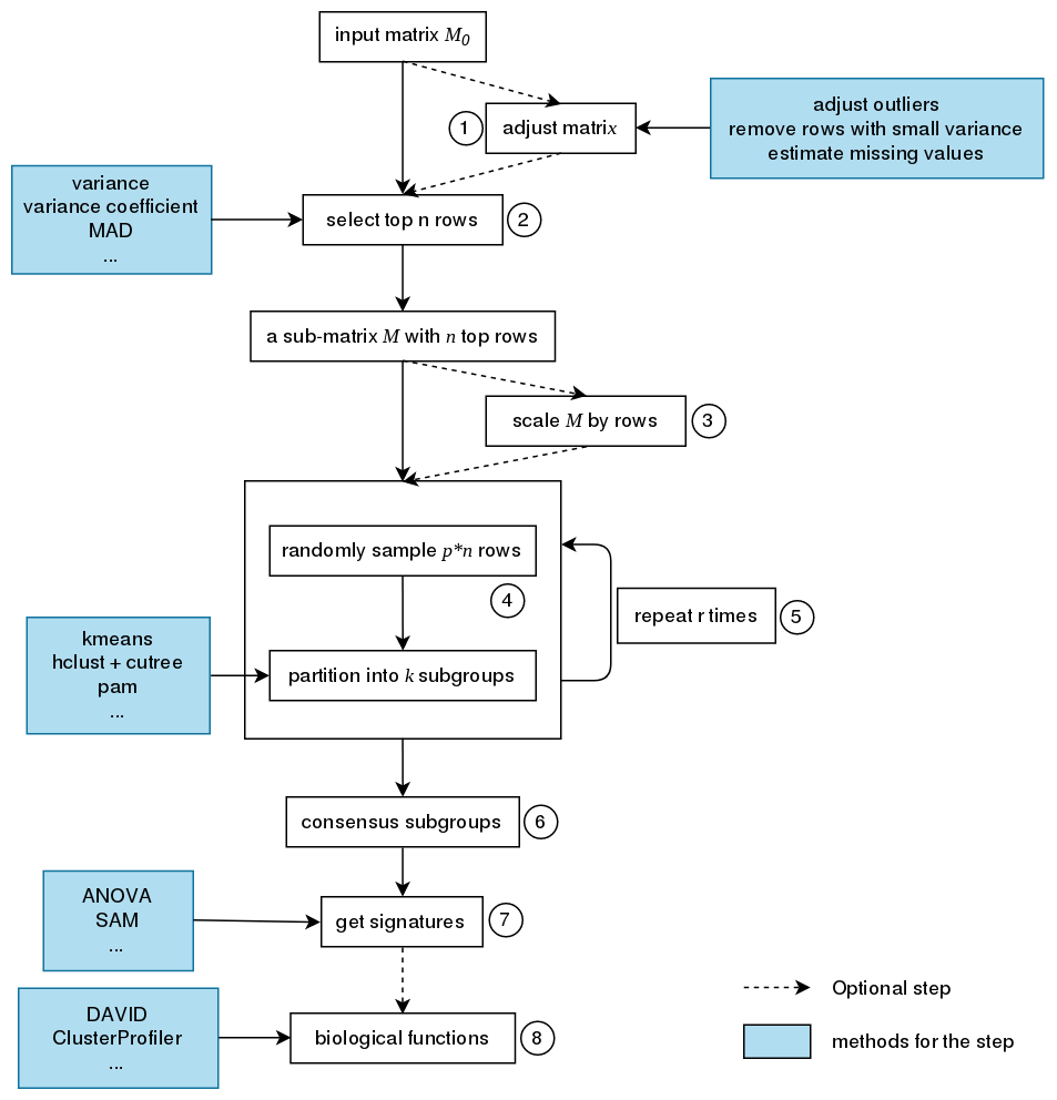
The steps of consensus partitioning is:

1. Clean the input matrix. The processing are: adjusting outliers, imputing missing values and removing rows with very small variance. This step is optional.
2. Extract subset of rows with highest scores. Here "scores" are calculated by a certain method. For gene expression analysis or methylation data analysis, $n$ rows with highest variance are used in most cases, where the "method", or let's call it "the top-value method" is the variance (by var() or sd()). Note the choice of "the top-value method" can be general. It can be e.g. MAD (median absolute deviation) or any user-defined method.
3. Scale the rows in the sub-matrix (e.g. gene expression) or not (e.g. methylation data). This step is optional.
4. Randomly sample a subset of rows from the sub-matrix with probability $p$ and perform partition on the columns of the matrix by a certain partition method, with trying different numbers of subgroups.
5. Repeat step 4 several times and collect all the partitions.
6. Perform consensus partitioning analysis and determine the best number of subgroups which gives the most stable subgrouping.
7. Apply statistical tests to find rows that show significant difference between the predicted subgroups. E.g. to extract subgroup specific genes.
8. If rows in the matrix can be associated to genes, downstream analysis such as function enrichment analysis can be performed.

Usage

Three lines of code to perfrom cola analysis:

mat = adjust_matrix(mat) # optional
rl = run_all_consensus_partition_methods(
    mat, 
    top_value_method = c("SD", "MAD", ...),
    partition_method = c("hclust", "kmeans", ...),
    mc.cores = ...)
cola_report(rl, output_dir = ...)

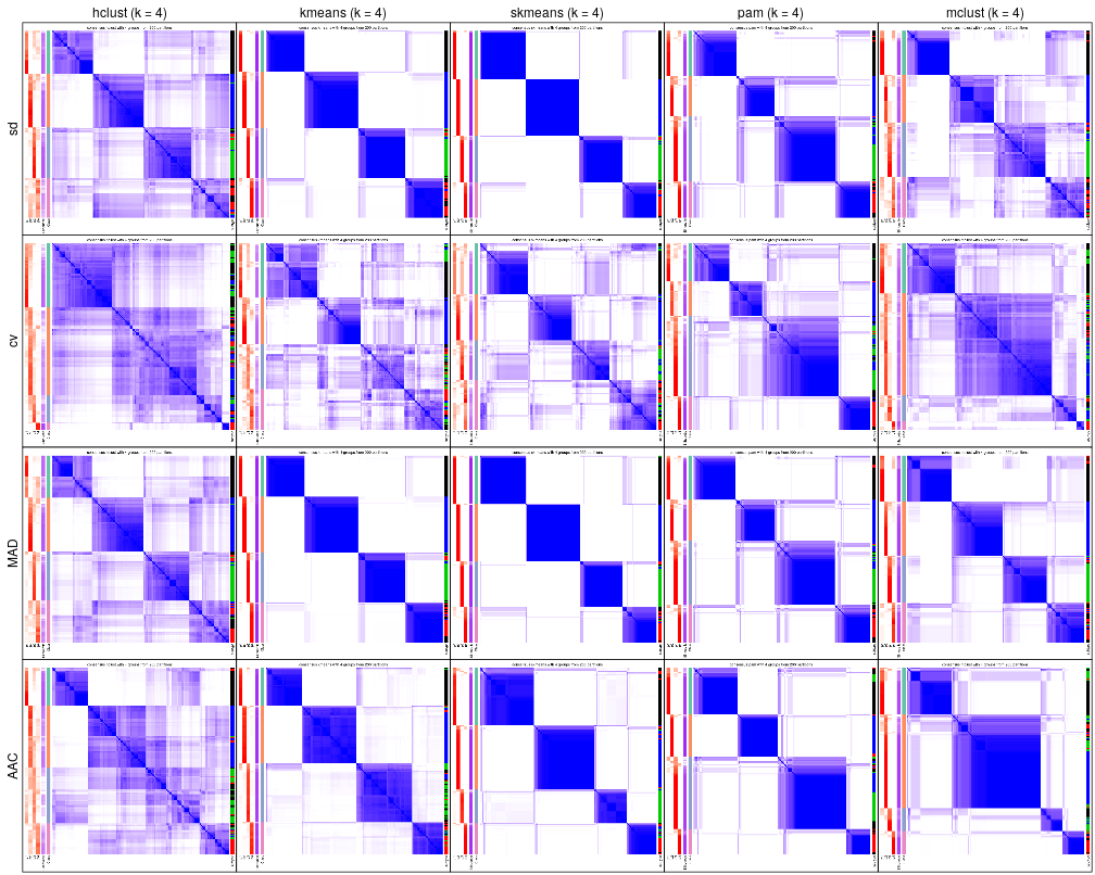
Plots

Following plots compare consensus heatmaps with k = 4 under all combinations of methods.

License

MIT @ Zuguang Gu

Acknowledgement

The cola icon in logo is made by photo3idea_studio from www.flaticon.com.

cola documentation built on Nov. 8, 2020, 8:12 p.m.