Nothing
ctsGE Package
In ctsGE: Clustering of Time Series Gene Expression data
library(ctsGE)
library(pander)
library(rmarkdown)
Installing ctsGE
if (!requireNamespace("BiocManager", quietly=TRUE))
    install.packages("BiocManager")
BiocManager::install("ctsGE")
Workflow of clustering with ctsGE
-
Build the expression matrix from expression data
-
Define an expression index (i.e., a sequence of 1,-1, and 0) for each gene
-
Cluster the gene set with the same index, applying K-means:
$$kmeans(genesInIndex,k)$$
-
Graphic visualization of expression patterns
-
Interactive visualization and exploration of gene-expression data
Building the expression matrix
As input, the ctsGE package expects a normalized expression table, where
rows are genes and columns are samples. This can consist of count data as
obtained, e. g., from RNA-Seq or other high-throughput sequencing experiment or
microarray experiment. Example data from the [Gene Expression Omnibus (GEO)]
(http://www.ncbi.nlm.nih.gov/geo/query/acc.cgi?acc=GSE2077) are used here
illustrate ctsGE's potential. The data are the expression profile of
Cryptosporidium parvum-infected human ileocecal adenocarcinoma cells
(HCT-8),^[Deng M, Lancto CA, Abrahamsen MS (2004).
Cryptosporidium parvum regulation of human epithelial cell gene expression.
Int. J. Parasitol. 34, 73–82.]) comprised of 12,625 genes over 18 samples
(three replicates of six developmental stages in human cancer). For tutorial
purposes and for simplification, only one replicate out of three is used,
for six overall time points.
Loading data from ncbi GEO
Load the files and make a list of the matrix:
When reading the normalized expression values the function check whether there
are rows that their median absolute deviation (MAD) value equal to zero and
remove these rows. This step is important in order to continue to the next step
of indexing the data.
library(GEOquery)

gse2077 <- getGEO('GSE2077')
gseAssays <- Biobase::assayData(gse2077)
gseExprs <- Biobase::assayDataElement(gseAssays[[1]][,c(1:6)],'exprs')

# list of the time series tables use only 6 samples
gseList <- lapply(1:6,function(x){data.frame(Genes = rownames(gseExprs),Value = gseExprs[,x])})
names(gseList) <- colnames(gseExprs)
Build the expression matrix from the list of matrices:
rts <- readTSGE(gseList,labels = c("0h","6h","12h","24h","48h","72h"))
Loading data from files
Here is an example of how to load the time-series files from your directory;
data were imported from the ctsGE package:
data_dir <- system.file("extdata", package = "ctsGE")
files <- dir(path=data_dir,pattern = "\\.xls$")
Building from a directory:
rts <- readTSGE(files, path = data_dir, labels = c("0h","6h","12h","24h","48h","72h") )
ctsGE Object summary:
names(rts)
rts$timePoints
head(rts$samples)
head(rts$tags)
head(rts$tsTable)
panderOptions("table.style","rmarkdown")
pander(head(rts$tsTable))
Adding genes annotation to time series table
Please use the desc option in the function: readTSGE in order to add genes
annotation to the time series table.
Defining the expression index
-
First, the expression matrix is standardized. The function default
standardizing method is a median-based scaling; alternatively, a mean-based
scaling can be used. The new scaled values represent the distance of each gene
at a certain time point from its center, median or mean, in median absolute
deviation (MAD) units or standard deviation (SD) units, respectively.
-
Next, the standardized values are converted to index values that indicate
whether gene expression is above, below or within the limits around the center
of the time series, i.e., 1 / -1 / 0, respectively. The function defines a
parameter cutoff (see Section 4.1) that
determines the limits around the gene-expression center.Then the function
calculates the index value at each time point according to:
- 0: standardized value is within the limits (+/- cutoff)
- 1: standardized value exceeds the upper limit (+ cutoff)
- -1: standardized value exceeds the lower limit (- cutoff)
-
The +/- cutoff parameter defines a reference range to which the data are
compared. When the range is too big, more time-series points will fall into
it and will get an index value of 0, and this may be misleading. Too small range
can result in too many index groups that will be too sensitive to small
fluctuations in the time-series index. The function chooses
the optimal cutoff (see Section 4.1) after
testing different cutoff values from 0.5 to 0.7 in increments of 0.05.
Checking the optimal cutoff
The function PreparingTheIndexes generates an expression index
(i.e., a sequence of 1,-1, and 0) that represents the expression pattern along
time points for each gene. Setting different limits for the center era
(with the parameter cutoff) will change the index for each gene-expression
profile and consequently, the number of genes in each index group. Following the
idea that instead of filtering “irrelevant” genes to reduce the noise, the
clustering will be performed on small gene groups, one would like to choose a
cutoff value, that will minimize the number of genes in each group, i.e.,
generate index groups of equal size. The test for equality is performed by
calculating the chi-squared value from a comparison between the number of genes
in the index groups and the null hypothesis that all index groups are equal.
The test is performed for all the cutoffs in the range and the cutoff that gives
the minimal chi-squared value is the most likely to generate equal index groups.
The range of the cutoff values is given by min_cutoff and max_cutoff
arguments. However, by setting the same value to min and max parameters one can
define a cutoff regardless of what was suggested by the function.
prts <- PreparingTheIndexes(x = rts, min_cutoff=0.5, max_cutoff=0.7, mad.scale = TRUE)
cutoff = 0.55 is the optimal cutoff with the lowest chi-squared value
prts$cutoff
Index overview after
To get an idea of how the data look, and to determine the nature of the indexes
formed from certain cutoff value, the number of zero values for each index
is counted. In this tutorial example, the index can have no zeros,
one zero or up to six zeros; overall, the indexes and genes are divided into
seven groups. Indexes for which most of the time points present a zero value
(in this example, three or more time points) are expected to show a pattern in
which gene-expression does not change much along the time points. Indexes with
less zeros to no zeros (two or less in the example) will show genes with up- or
downregulated expression at each time point.
With cutoff =
0.55, most of the genes were assigned to indexes with three or two zeros,
indicating a variety of expression patterns.
library(dplyr)

count_zero <-
  function(x){
    sum(strsplit(x,"")[[1]]==0)}


tbl <- prts$index %>%
    # counting genes at each index
    group_by(index)%>% summarise(size=length(index)) %>%
    # counting the number of zeros at each index
    group_by(index)%>% mutate(nzero=count_zero(as.character(index))) %>%
    # groups genes by the number of zeros and sum them
    group_by(nzero) %>% summarise(genes=round(sum(size)/12625,1))

tmp = which(0:6%in%tbl$nzero==0)-1
tmp_df = data.frame(nzero=tmp,genes=rep(0,length(tmp)))
tbl <- bind_rows(tbl,tmp_df) %>% arrange(nzero)
labs <- seq(0,max(tbl$genes), by = 0.2)
barplot(tbl$genes,
        main = paste("Number of zeros in indexes with cutoff =",prts$cutoff),
        names.arg = tbl$nzero,axes = FALSE, xlab="Number of Zeros")
axis(side = 2, at = labs, labels = paste0(labs * 100, "%"))
Preparing the indexes for the data
A cutoff = 0.55 was chosen
prts <- PreparingTheIndexes(x = rts, mad.scale = TRUE)
names(prts)
Gene expression after standardization:
head(prts$scaled)
panderOptions("table.style","simple")
pander(head(prts$scaled))
Gene expression indexing with cutoff = 0.55:
head(prts$index)
panderOptions("table.style","simple")
pander(head(prts$index))
Clustering each index with K-means
The clustering is done with K-means. To choose an optimal k for K-means
clustering, the Elbow method was applied^[Thorndike RL (1953). Who Belongs in
the Family? Psychometrika, 18(4), 267–276.], this method looks at the percentage
of variance explained as a function of the number of clusters: the chosen number
of clusters should be such that adding another cluster does not give much better
modeling of the data. First, the ratio of the within-cluster sum of squares
(WSS) to the total sum of squares (TSS) is computed for different values of
k (i.e., 1, 2, 3 ...). The WSS, also known as sum of squared error (SSE),
decreases as k gets larger. The Elbow method chooses the k at which the SSE
decreases abruptly. This happens when the computed value of the WSS-to-TSS ratio
first drops from 0.2.
$\frac{WSS}{TSS} < 0.2$
ClustIndexes <- ClustIndexes(prts, scaling = TRUE)
names(ClustIndexes)
# table of the index and the recommended k that were found by the function
head(ClustIndexes$optimalK)

# Table of clusters index for each gene
head(ClustIndexes$ClusteredIdxTable)
Running kmeans and calculating the optimal k for each one of the indexes in
the data could take a long time. To shorten the procedure the user can skip this
step altogether and directly view a specific index and its clusters by running either
the PlotIndexesClust() or the ctsGEShinyApp() function
Graphic visualization of an index
The PlotIndexesClust() function generates graphs and tables of a specific
index and its clusters. The user decides whether to supply the k or let the
function calculate the k for the selected index.
indexPlot <- PlotIndexesClust(prts,idx = "1100-1-1",scaling = TRUE)
names(indexPlot)
Genes in '1100-1-1' index and their clusters
(k was chosen by the function):
Number of clusters (k) for '1100-1-1' is: length(indexPlot$graphs)
length(indexPlot$graphs)
Table of genes in '1100-1-1' index, seperated to clusters:
head(indexPlot[[1]])
panderOptions("table.style","rmarkdown")
pander(head(indexPlot[[1]]))
For this example, the index 1100-1-1 is used. by Looking at this index, it can
be assumed that the expression of the genes belonging to it was downregulated
along the time points. Since the index only states whether gene expression
is upregulated (1), downregulated (-1) or stays the same (0), gene subsets
of the same profile will usually show more than one expression pattern.
K-means helps distinguish these patterns from one another.
Line graphs of the genes' expression patterns in index '1100-1-1' separated
into clusters:
indexPlot$graphs
Export gene expression table to file
Genes expression data in index '1100-1-1' separated into clsuter can be
exported with R function write.table:
write.table(indexPlot[[1]], file, sep = "\t")
GUI for interactive exploration of gene-expression data
The ctsGEShinyApp function the ctsGE object,and opens an html page as a GUI.
On the web page, the user chooses the profile to visualize and the number of
clusters (k parameter for K-means) to show. The line graph of the profile
separated into the clusters will show in the main panel, and a list of the genes
and their expressions will also be available. The tables and figures can be
downloaded.
*Note that running the Shiny GUI block the current session while running.
Screenshots of the GUI
library(shiny)
library(DT)
ctsGEShinyApp(rts)
The graph tab
The table tab
Try the ctsGE package in your browser
Any scripts or data that you put into this service are public.
ctsGE documentation built on Nov. 8, 2020, 11:06 p.m.
R Package Documentation
Browse R Packages
We want your feedback!
Note that we can't provide technical support on individual packages. You should contact the package authors for that.
library(ctsGE) library(pander) library(rmarkdown)
Installing ctsGE
if (!requireNamespace("BiocManager", quietly=TRUE)) install.packages("BiocManager") BiocManager::install("ctsGE")
Workflow of clustering with ctsGE
-
Build the expression matrix from expression data
-
Define an expression index (i.e., a sequence of 1,-1, and 0) for each gene
-
Cluster the gene set with the same index, applying K-means: $$kmeans(genesInIndex,k)$$
-
Graphic visualization of expression patterns
-
Interactive visualization and exploration of gene-expression data
Building the expression matrix
As input, the ctsGE package expects a normalized expression table, where rows are genes and columns are samples. This can consist of count data as obtained, e. g., from RNA-Seq or other high-throughput sequencing experiment or microarray experiment. Example data from the [Gene Expression Omnibus (GEO)] (http://www.ncbi.nlm.nih.gov/geo/query/acc.cgi?acc=GSE2077) are used here illustrate ctsGE's potential. The data are the expression profile of Cryptosporidium parvum-infected human ileocecal adenocarcinoma cells (HCT-8),^[Deng M, Lancto CA, Abrahamsen MS (2004). Cryptosporidium parvum regulation of human epithelial cell gene expression. Int. J. Parasitol. 34, 73–82.]) comprised of 12,625 genes over 18 samples (three replicates of six developmental stages in human cancer). For tutorial purposes and for simplification, only one replicate out of three is used, for six overall time points.
Loading data from ncbi GEO
Load the files and make a list of the matrix:
When reading the normalized expression values the function check whether there are rows that their median absolute deviation (MAD) value equal to zero and remove these rows. This step is important in order to continue to the next step of indexing the data.
library(GEOquery) gse2077 <- getGEO('GSE2077') gseAssays <- Biobase::assayData(gse2077) gseExprs <- Biobase::assayDataElement(gseAssays[[1]][,c(1:6)],'exprs') # list of the time series tables use only 6 samples gseList <- lapply(1:6,function(x){data.frame(Genes = rownames(gseExprs),Value = gseExprs[,x])}) names(gseList) <- colnames(gseExprs)
Build the expression matrix from the list of matrices:
rts <- readTSGE(gseList,labels = c("0h","6h","12h","24h","48h","72h"))
Loading data from files
Here is an example of how to load the time-series files from your directory; data were imported from the ctsGE package:
data_dir <- system.file("extdata", package = "ctsGE") files <- dir(path=data_dir,pattern = "\\.xls$")
Building from a directory:
rts <- readTSGE(files, path = data_dir, labels = c("0h","6h","12h","24h","48h","72h") )
ctsGE Object summary:
names(rts) rts$timePoints head(rts$samples) head(rts$tags)
head(rts$tsTable)
panderOptions("table.style","rmarkdown") pander(head(rts$tsTable))
Adding genes annotation to time series table
Please use the desc option in the function: readTSGE in order to add genes
annotation to the time series table.
Defining the expression index
-
First, the expression matrix is standardized. The function default standardizing method is a median-based scaling; alternatively, a mean-based scaling can be used. The new scaled values represent the distance of each gene at a certain time point from its center, median or mean, in median absolute deviation (MAD) units or standard deviation (SD) units, respectively.
-
Next, the standardized values are converted to index values that indicate whether gene expression is above, below or within the limits around the center of the time series, i.e., 1 / -1 / 0, respectively. The function defines a parameter cutoff (see Section 4.1) that determines the limits around the gene-expression center.Then the function calculates the index value at each time point according to:
- 0: standardized value is within the limits (+/- cutoff)
- 1: standardized value exceeds the upper limit (+ cutoff)
- -1: standardized value exceeds the lower limit (- cutoff)
-
The
+/- cutoffparameter defines a reference range to which the data are compared. When the range is too big, more time-series points will fall into it and will get an index value of 0, and this may be misleading. Too small range can result in too many index groups that will be too sensitive to small fluctuations in the time-series index. The function chooses the optimal cutoff (see Section 4.1) after testing different cutoff values from 0.5 to 0.7 in increments of 0.05.
Checking the optimal cutoff
The function PreparingTheIndexes generates an expression index
(i.e., a sequence of 1,-1, and 0) that represents the expression pattern along
time points for each gene. Setting different limits for the center era
(with the parameter cutoff) will change the index for each gene-expression
profile and consequently, the number of genes in each index group. Following the
idea that instead of filtering “irrelevant” genes to reduce the noise, the
clustering will be performed on small gene groups, one would like to choose a
cutoff value, that will minimize the number of genes in each group, i.e.,
generate index groups of equal size. The test for equality is performed by
calculating the chi-squared value from a comparison between the number of genes
in the index groups and the null hypothesis that all index groups are equal.
The test is performed for all the cutoffs in the range and the cutoff that gives
the minimal chi-squared value is the most likely to generate equal index groups.
The range of the cutoff values is given by min_cutoff and max_cutoff
arguments. However, by setting the same value to min and max parameters one can
define a cutoff regardless of what was suggested by the function.
prts <- PreparingTheIndexes(x = rts, min_cutoff=0.5, max_cutoff=0.7, mad.scale = TRUE)
cutoff = 0.55 is the optimal cutoff with the lowest chi-squared value
prts$cutoff
Index overview after
To get an idea of how the data look, and to determine the nature of the indexes formed from certain cutoff value, the number of zero values for each index is counted. In this tutorial example, the index can have no zeros, one zero or up to six zeros; overall, the indexes and genes are divided into seven groups. Indexes for which most of the time points present a zero value (in this example, three or more time points) are expected to show a pattern in which gene-expression does not change much along the time points. Indexes with less zeros to no zeros (two or less in the example) will show genes with up- or downregulated expression at each time point.
With cutoff = 0.55, most of the genes were assigned to indexes with three or two zeros, indicating a variety of expression patterns.
library(dplyr) count_zero <- function(x){ sum(strsplit(x,"")[[1]]==0)} tbl <- prts$index %>% # counting genes at each index group_by(index)%>% summarise(size=length(index)) %>% # counting the number of zeros at each index group_by(index)%>% mutate(nzero=count_zero(as.character(index))) %>% # groups genes by the number of zeros and sum them group_by(nzero) %>% summarise(genes=round(sum(size)/12625,1)) tmp = which(0:6%in%tbl$nzero==0)-1 tmp_df = data.frame(nzero=tmp,genes=rep(0,length(tmp))) tbl <- bind_rows(tbl,tmp_df) %>% arrange(nzero) labs <- seq(0,max(tbl$genes), by = 0.2) barplot(tbl$genes, main = paste("Number of zeros in indexes with cutoff =",prts$cutoff), names.arg = tbl$nzero,axes = FALSE, xlab="Number of Zeros") axis(side = 2, at = labs, labels = paste0(labs * 100, "%"))
Preparing the indexes for the data
A cutoff = 0.55 was chosen
prts <- PreparingTheIndexes(x = rts, mad.scale = TRUE) names(prts)
Gene expression after standardization:
head(prts$scaled)
panderOptions("table.style","simple") pander(head(prts$scaled))
Gene expression indexing with cutoff = 0.55:
head(prts$index)
panderOptions("table.style","simple") pander(head(prts$index))
Clustering each index with K-means
The clustering is done with K-means. To choose an optimal k for K-means clustering, the Elbow method was applied^[Thorndike RL (1953). Who Belongs in the Family? Psychometrika, 18(4), 267–276.], this method looks at the percentage of variance explained as a function of the number of clusters: the chosen number of clusters should be such that adding another cluster does not give much better modeling of the data. First, the ratio of the within-cluster sum of squares (WSS) to the total sum of squares (TSS) is computed for different values of k (i.e., 1, 2, 3 ...). The WSS, also known as sum of squared error (SSE), decreases as k gets larger. The Elbow method chooses the k at which the SSE decreases abruptly. This happens when the computed value of the WSS-to-TSS ratio first drops from 0.2.
$\frac{WSS}{TSS} < 0.2$
ClustIndexes <- ClustIndexes(prts, scaling = TRUE) names(ClustIndexes) # table of the index and the recommended k that were found by the function head(ClustIndexes$optimalK) # Table of clusters index for each gene head(ClustIndexes$ClusteredIdxTable)
Running kmeans and calculating the optimal k for each one of the indexes in
the data could take a long time. To shorten the procedure the user can skip this
step altogether and directly view a specific index and its clusters by running either
the PlotIndexesClust() or the ctsGEShinyApp() function
Graphic visualization of an index
The PlotIndexesClust() function generates graphs and tables of a specific
index and its clusters. The user decides whether to supply the k or let the
function calculate the k for the selected index.
indexPlot <- PlotIndexesClust(prts,idx = "1100-1-1",scaling = TRUE) names(indexPlot)
Genes in '1100-1-1' index and their clusters
(k was chosen by the function):
Number of clusters (k) for '1100-1-1' is: length(indexPlot$graphs)
length(indexPlot$graphs)
Table of genes in '1100-1-1' index, seperated to clusters:
head(indexPlot[[1]])
panderOptions("table.style","rmarkdown") pander(head(indexPlot[[1]]))
For this example, the index 1100-1-1 is used. by Looking at this index, it can
be assumed that the expression of the genes belonging to it was downregulated
along the time points. Since the index only states whether gene expression
is upregulated (1), downregulated (-1) or stays the same (0), gene subsets
of the same profile will usually show more than one expression pattern.
K-means helps distinguish these patterns from one another.
Line graphs of the genes' expression patterns in index '1100-1-1' separated into clusters:
indexPlot$graphs
Export gene expression table to file
Genes expression data in index '1100-1-1' separated into clsuter can be
exported with R function write.table:
write.table(indexPlot[[1]], file, sep = "\t")
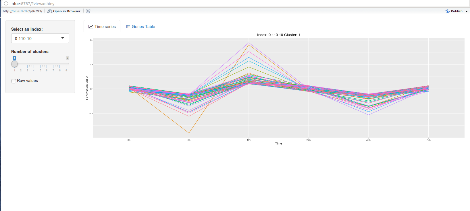
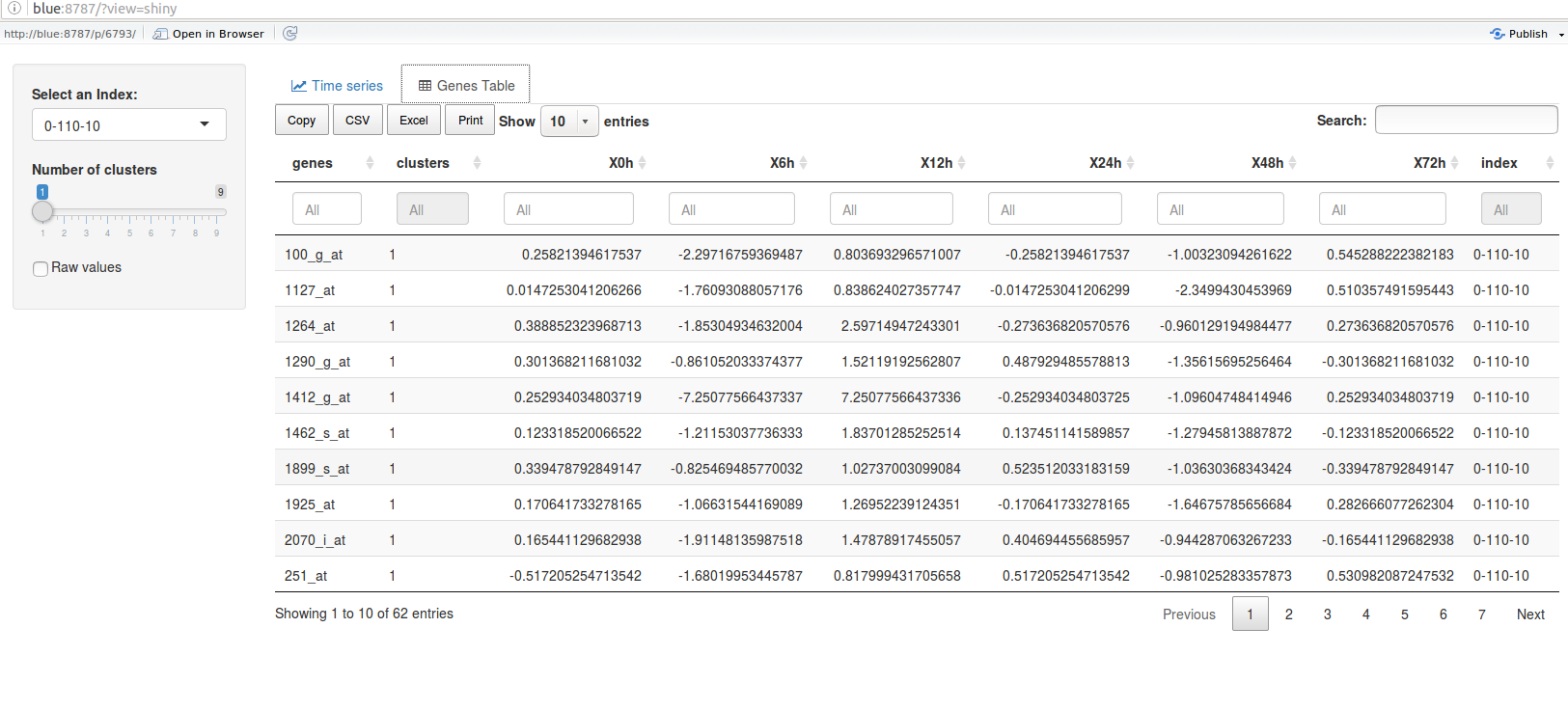
GUI for interactive exploration of gene-expression data
The ctsGEShinyApp function the ctsGE object,and opens an html page as a GUI.
On the web page, the user chooses the profile to visualize and the number of
clusters (k parameter for K-means) to show. The line graph of the profile
separated into the clusters will show in the main panel, and a list of the genes
and their expressions will also be available. The tables and figures can be
downloaded.
*Note that running the Shiny GUI block the current session while running.
Screenshots of the GUI
library(shiny) library(DT) ctsGEShinyApp(rts)
The graph tab
The table tab
Try the ctsGE package in your browser
Any scripts or data that you put into this service are public.
R Package Documentation
Browse R Packages
We want your feedback!
Note that we can't provide technical support on individual packages. You should contact the package authors for that.
Embedding an R snippet on your website
Add the following code to your website.
For more information on customizing the embed code, read Embedding Snippets.