README.md
In IDF: Estimation and Plotting of IDF Curves

IDF

Intensity-duration-frequency (IDF) curves are a widely used analysis-tool in hydrology to assess the characteristics of extreme precipitation. The package ‘IDF’ functions to estimate IDF relations for given precipitation time series on the basis of a duration-dependent generalized extreme value (GEV) distribution. The central function is , which uses the method of maximum-likelihood estimation for the d-GEV parameters, whereby it is possible to include generalized linear modeling for each parameter. For more detailed information on the methods and the application of the package for estimating IDF curves with spatial covariates, see Ulrich et. al (2020, https://doi.org/10.3390/w12113119).

You can install the released version of IDF from CRAN with:

install.packages("IDF")

or from gitlab using:

devtools::install_git("https://gitlab.met.fu-berlin.de/Rpackages/idf_package")

Here are a few examples to illustrate the order in which the functions are intended to be used.

Step 0: sample 20 years of example hourly ‘precipitation’ data

set.seed(999)
dates <- seq(as.POSIXct("2000-01-01 00:00:00"),as.POSIXct("2019-12-31 23:00:00"),by = 'hour')
sample.precip <- rgamma(n = length(dates), shape = 0.05, rate = 0.4)
precip.df <- data.frame(date=dates,RR=sample.precip)

Step 1: get annual maxima

library(IDF)

durations <- 2^(0:6) # accumulation durations [h] 
ann.max <- IDF.agg(list(precip.df),ds=durations,na.accept = 0.1)
# plotting the annual maxima in log-log representation
plot(ann.max$ds,ann.max$xdat,log='xy',xlab = 'Duration [h]',ylab='Intensity [mm/h]')

Step 2: fit d-GEV to annual maxima

fit <- gev.d.fit(xdat = ann.max$xdat,ds = ann.max$ds,sigma0link = make.link('log'))
#> $conv
#> [1] 0
#> 
#> $nllh
#> [1] 59.34496
#> 
#> $mle
#> [1]  6.478887e+00  3.817184e-01 -1.833254e-02  2.843666e-09  7.922310e-01
#> 
#> $se
#> [1] 0.25207846 0.02370771 0.04861600        NaN 0.01008561
# checking the fit 
gev.d.diag(fit,pch=1,ci=TRUE)

# parameter estimates 
params <- gev.d.params(fit)
print(params)
#>        mut sigma0          xi        theta      eta eta2 tau
#> 1 6.478887 1.4648 -0.01833254 2.843666e-09 0.792231    0   0

# plotting the probability density for a single duration 
q.min <- floor(min(ann.max$xdat[ann.max$ds%in%1:2]))
q.max <- ceiling(max(ann.max$xdat[ann.max$ds%in%1:2]))
q <- seq(q.min,q.max,0.2)
plot(range(q),c(0,0.55),type = 'n',xlab = 'Intensity [mm/h]',ylab = 'Density')
for(d in 1:2){ # d=1h and d=2h
  # sampled data:
  hist(ann.max$xdat[ann.max$ds==d],main = paste('d=',d),q.min:q.max
       ,freq = FALSE,add=TRUE,border = d)   
  # etimated prob. density:
  lines(q,dgev.d(q,params$mut,params$sigma0,params$xi,params$theta,params$eta,params$tau,d = d),col=d) 
}
legend('topright',col=1:2,lwd=1,legend = paste('d=',1:2,'h'),title = 'Duration')

Step 3: adding the IDF-curves to the data

plot(ann.max$ds,ann.max$xdat,log='xy',xlab = 'Duration [h]',ylab='Intensity [mm/h]')
IDF.plot(durations,params,add=TRUE)

This Example depicts the different features that can be used to model the IDF curves, see Fauer et. al (2021, https://doi.org/10.5194/hess-25-6479-2021). Here we assume, that the block maxima of each duration can be modeled with the GEV distribution ( $\xi\neq0$ ):

$G(z;\mu,\sigma,\xi)=\exp \left\lbrace -\left[ 1+\xi \left( \frac{z-\mu}{\sigma} \right) \right]^{-1/\xi} \right\rbrace,$

where the GEV parameters depend on duration according to:

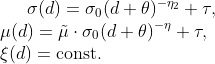
$\sigma(d)=\sigma_0(d+\theta)^{-\eta_2}+\tau, \\ \mu(d) = \tilde{\mu}\cdot\sigma_0(d+\theta)^{-\eta}+\tau, \\ \xi(d) = \text{const.}$

The function gev.d.fit provides the options:

theta_zero = TRUE $\theta = 0$
eta2_zero = TRUE (default) $\eta_2 = \eta$
tau_zero = TRUE (default) $\tau = 0$

resulting in the following features for IDF-curves:

simple scaling: using only parameters $\tilde{\mu}, \sigma_0, \xi, \eta$
curvature for small durations: allowing $\theta \neq 0$ (default)
multi-scaling: allowing $\eta_2 \neq \eta$
flattening for long durations: allowing $\tau \neq 0$ .

Example:

### sampling example data
set.seed(42)
# durations
ds <- 1/60*2^(seq(0,13,1))
# random data for each duration
xdat <- sapply(ds,rgev.d,n = 20,mut = 2,sigma0 =3,xi = 0.2,theta = 0.1,eta = 0.6,tau = 0.1,eta2 = 0.2)
# transform to data.frame
example <- data.frame(xdat=as.numeric(xdat),ds=rep(ds,each=dim(xdat)[1]))

### different fit options
fit.simple <- gev.d.fit(xdat=example$xdat,ds = example$ds,theta_zero = TRUE,show=FALSE)
fit.theta <- gev.d.fit(xdat=example$xdat,ds = example$ds,show=FALSE)
fit.eta2 <- gev.d.fit(xdat=example$xdat,ds = example$ds,eta2_zero = FALSE,show=FALSE)
fit.tau <- gev.d.fit(xdat=example$xdat,ds = example$ds,eta2_zero = FALSE,tau_zero = FALSE,show=FALSE)
# group fits
all.fits <- list(simple=fit.simple,curvature=fit.theta,multiscaling=fit.eta2,flattening=fit.tau)
# compare parameter estimates:
print(t(sapply(all.fits,gev.d.params)))
#>              mut      sigma0   xi           theta      eta       eta2     
#> simple       1.754974 2.897875 -0.004559432 0          0.4978471 0        
#> curvature    1.782777 3.187756 -0.01039414  0.02949747 0.5376237 0        
#> multiscaling 1.896368 2.826447 0.1358611    0.03034914 0.4971133 0.1577612
#> flattening   2.038391 2.712067 0.1469354    0.09235748 0.6237206 0.2642782
#>              tau      
#> simple       0        
#> curvature    0        
#> multiscaling 0        
#> flattening   0.1287691

### compare resulting idf-curves
fit.cols <- c('red','purple','blue','darkgreen')
fit.labels <- c('simple-scaling','theta!=0','eta2!=eta','tau!=0')
# plotting probabilities
idf.probs <- c(0.5,0.75,0.99) 
# create 4 plots: one for each additional parameter
par(mfrow=c(2,2),mar=c(0.2,0.2,0.2,0.2),oma=c(3.5,4.5,0,0),mgp=c(2.5,0.6,0))
for(i.fit in 1:length(all.fits)){
  plot(example$ds,example$xdat,log='xy',type='n',axes=FALSE)
  box()
  boxplot(example$xdat~example$ds,at=ds,add = TRUE,
        boxwex=0.2,cex=0.4,axes=FALSE)
  if(i.fit %in% c(1,3)){
    axis(2,las=2)
    mtext('Intensity [mm/h]',2,3)
  }
  if(i.fit %in% 3:4){
    axis(1,at=c(0.1,1,24,120),labels = c(0.1,1,24,120))
    mtext('Duration [h]',1,2)
  }
  for(i.p in 1:length(idf.probs)){
    # plotting IDF curves for each model (different colors) and probability (different lty)
    IDF.plot(1/60*2^(seq(0,13,0.5)),gev.d.params(all.fits[[i.fit]]),probs = idf.probs[i.p]
             ,add = TRUE,legend = FALSE,lty = i.p,cols = fit.cols[i.fit])
  }
  mtext(fit.labels[i.fit],3,-1.25)
}
legend('topright',lty=rev(1:3),legend = rev(idf.probs),title = 'p-quantile')