Nothing
Solving Delay Differential Equations (DDE) in R with diffeqr
In diffeqr: Solving Differential Equations (ODEs, SDEs, DDEs, DAEs)
knitr::opts_chunk$set(
  collapse = TRUE,
  comment = "#>"
)
A delay differential equation is an ODE which allows the use of previous values. In this case, the function
needs to be a JIT compiled Julia function. It looks just like the ODE, except in this case there is a function
h(p,t) which allows you to interpolate and grab previous values.
We must provide a history function h(p,t) that gives values for u before
t0. Here we assume that the solution was constant before the initial time point. Additionally, we pass
constant_lags = c(20.0) to tell the solver that only constant-time lags were used and what the lag length
was. This helps improve the solver accuracy by accurately stepping at the points of discontinuity. Together
this is:
f <- JuliaCall::julia_eval("function f(du, u, h, p, t)
  du[1] = 1.1/(1 + sqrt(10)*(h(p, t-20)[1])^(5/4)) - 10*u[1]/(1 + 40*u[2])
  du[2] = 100*u[1]/(1 + 40*u[2]) - 2.43*u[2]
end")
h <- JuliaCall::julia_eval("function h(p, t)
  [1.05767027/3, 1.030713491/3]
end")
u0 <- c(1.05767027/3, 1.030713491/3)
tspan <- c(0.0, 100.0)
constant_lags <- c(20.0)
JuliaCall::julia_assign("u0", u0)
JuliaCall::julia_assign("tspan", tspan)
JuliaCall::julia_assign("constant_lags", tspan)
prob <- JuliaCall::julia_eval("DDEProblem(f, u0, h, tspan, constant_lags = constant_lags)")
sol <- de$solve(prob,de$MethodOfSteps(de$Tsit5()))
udf <- as.data.frame(t(sapply(sol$u,identity)))
plotly::plot_ly(udf, x = sol$t, y = ~V1, type = 'scatter', mode = 'lines') %>% plotly::add_trace(y = ~V2)
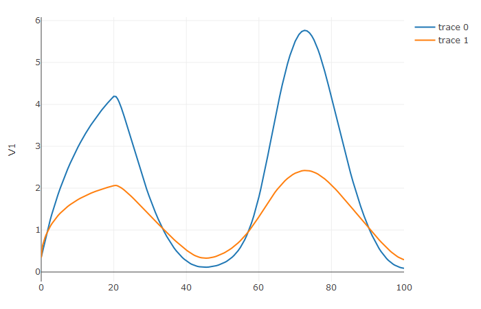
Notice that the solver accurately is able to simulate the kink (discontinuity) at t=20 due to the discontinuity
of the derivative at the initial time point! This is why declaring discontinuities can enhance the solver accuracy.
Try the diffeqr package in your browser
Any scripts or data that you put into this service are public.
diffeqr documentation built on April 3, 2025, 10:21 p.m.
R Package Documentation
Browse R Packages
We want your feedback!
Note that we can't provide technical support on individual packages. You should contact the package authors for that.
knitr::opts_chunk$set( collapse = TRUE, comment = "#>" )
A delay differential equation is an ODE which allows the use of previous values. In this case, the function
needs to be a JIT compiled Julia function. It looks just like the ODE, except in this case there is a function
h(p,t) which allows you to interpolate and grab previous values.
We must provide a history function h(p,t) that gives values for u before
t0. Here we assume that the solution was constant before the initial time point. Additionally, we pass
constant_lags = c(20.0) to tell the solver that only constant-time lags were used and what the lag length
was. This helps improve the solver accuracy by accurately stepping at the points of discontinuity. Together
this is:
f <- JuliaCall::julia_eval("function f(du, u, h, p, t) du[1] = 1.1/(1 + sqrt(10)*(h(p, t-20)[1])^(5/4)) - 10*u[1]/(1 + 40*u[2]) du[2] = 100*u[1]/(1 + 40*u[2]) - 2.43*u[2] end") h <- JuliaCall::julia_eval("function h(p, t) [1.05767027/3, 1.030713491/3] end") u0 <- c(1.05767027/3, 1.030713491/3) tspan <- c(0.0, 100.0) constant_lags <- c(20.0) JuliaCall::julia_assign("u0", u0) JuliaCall::julia_assign("tspan", tspan) JuliaCall::julia_assign("constant_lags", tspan) prob <- JuliaCall::julia_eval("DDEProblem(f, u0, h, tspan, constant_lags = constant_lags)") sol <- de$solve(prob,de$MethodOfSteps(de$Tsit5())) udf <- as.data.frame(t(sapply(sol$u,identity))) plotly::plot_ly(udf, x = sol$t, y = ~V1, type = 'scatter', mode = 'lines') %>% plotly::add_trace(y = ~V2)
Notice that the solver accurately is able to simulate the kink (discontinuity) at t=20 due to the discontinuity
of the derivative at the initial time point! This is why declaring discontinuities can enhance the solver accuracy.
Try the diffeqr package in your browser
Any scripts or data that you put into this service are public.
R Package Documentation
Browse R Packages
We want your feedback!
Note that we can't provide technical support on individual packages. You should contact the package authors for that.
Embedding an R snippet on your website
Add the following code to your website.
For more information on customizing the embed code, read Embedding Snippets.