Nothing
The Propensity to Cycle Tool
In pct: Propensity to Cycle Tool
# get citations
refs = RefManageR::ReadZotero(group = "418217", .params = list(collection = "JFR868KJ", limit = 100))
refs_df = as.data.frame(refs)
# View(refs_df)
# citr::insert_citation(bib_file = "vignettes/refs_training.bib")
RefManageR::WriteBib(refs, "refs.bib")
# citr::tidy_bib_file(rmd_file = "vignettes/pct_training.Rmd", messy_bibliography = "vignettes/refs_training.bib")
options(htmltools.dir.version = FALSE)
knitr::opts_chunk$set(message = FALSE)
library(RefManageR)
BibOptions(check.entries = FALSE,
           bib.style = "authoryear",
           cite.style = 'alphabetic',
           style = "markdown",
           first.inits = FALSE,
           hyperlink = FALSE,
           dashed = FALSE)
my_bib = refs
library(RefManageR)
my_bib = RefManageR::ReadBib("refs.bib")
# publish results online
cp -Rv inst/rmd/pct-slides* ~/saferactive/site/static/slides/
cp -Rv inst/rmd/libs ~/saferactive/site/static/slides/
cd ~/saferactive/site
git add -A
git status
git commit -am 'Update slides'
git push
cd -
Intro + agenda
This workshop will provide an overview of the PCT for advanced users, including:
- transport planners with experience of evidence-based prioritisation
- researchers with experience of using origin-destination, route and route network level data
- programmers, developers and others wanting to extend PCT methods for the public benefit
--
The workshop will be broken into three main parts:
Part 1: how the Propensity to Cycle Tool works + demo: 'I do' (14:00 - 15:00)
Part 2: Co-coding session: 'we do' (15:00 - 15:45)
☕☕☕ 15 minute break ☕☕☕
Part 3: using PCT data for your needs: 'you do' (16:00 - 17:00)
- Presentation of work and next steps (17:00 - 17:15)
- Networking and 'ideas with beers' 🍻🍻🍻 (17:20 - 18:00)
Description:
In this workshop you will take a deep dive into the Propensity to Cycle Tool (PCT).
Beginner and intermediate PCT events focus on using the PCT via the web application hosted at www.pct.bike and the data provided by the PCT in QGIS but the focus here is on analysing cycling potential in the open source statistical programming language R. The majority of the PCT was built on R, which is a powerful object-orientated programming language with a focus on statistical modelling, visualisation and geographic analysis. The workshop will show how the code underlying the PCT works, how the underlying data can be accessed for reproducible analysis, and how the methods can be used to generate new scenarios of cycling uptake.
Preparation
If you are inexperienced with R you should prepare by
- Essential: taking an online course such as the free 'Introduction to R' course provided by DataCamp
- Essential: ensuring you have installed up-to-date versions of R (R 4.0.0 or greater), RStudio (1.2 or greater) and the pct R package (0.6.0) on your computer
- Essential: test your computer set up by running the R code here github.com/ITSLeeds/pct/blob/master/inst/test-setup.R - you should make a note of the result of this final commented-out command:
round(mean(rnet_potential$Potential))
- Highly recommended: working through and reproducing results in Chapter 12 onwards of the open source book Geocomputation with R (see geocompr.robinlovelace.net/transport.html)
If you are new to R but have not completed the above tasks you may be unable to follow the second and third sections of the workshop outlined in the agenda below.
Prerequisites
See here for a guide on installing R and RStudio for transport data research.
To get the access code for the tutorial, you will need to first work through the code shown here:
https://github.com/ITSLeeds/pct/blob/master/inst/test-setup.R
After you have run the code, running the following line should give you a number that will give you the access code for the course:
round(mean(rnet_potential$Potential))
Save that 3 digit number, it will allow access to the workshop.
If you have any issues with your computer set-up, please ask a question here (you will need to sign-up for a GitHub account if you have not already done so): https://github.com/ITSLeeds/pct/issues/67
background-image: url(https://media.giphy.com/media/YlQQYUIEAZ76o/giphy.gif)
background-size: cover
class: center, middle
How the PCT works
The first prototype of the PCT
-
1st prototype: Hackathon at ODI Leeds in February 2015
-
We identifying key routes and mapped them
-
For description of aims, see Lovelace et al. (2017)
knitr::include_graphics("https://raw.githubusercontent.com/npct/pct-team/master/figures/early.png")
- Launched in 2017 with the Cycling and Walking Investment Strategy (CWIS)

Photo: demo of the PCT to Secretary of State for Transport (March 2017)
The PCT in 2020
- Now the go-to tool for strategic cycle network planning in England and Wales, used by most local authorities with cycling plans (source).
.pull-left[
Geographic levels in the PCT
- Generate and analyse route networks for transport planning with reference to:
- Zones
- Origin-destination (OD) data
- Geographic desire lines
- Route allocation using different routing services
- Route network generation and analysis
]
.pull-right[
 See these levels at www.pct.bike
]
Let's look at zones

qtm(od_data_zones_min)
MSOA vs LSOA zones (MSOA zones ~5 times bigger)
# not the best example
# knitr::include_graphics("https://user-images.githubusercontent.com/1825120/96573136-a1f55800-12c5-11eb-8921-c9938cd9e929.gif")
knitr::include_graphics(c(
  "https://user-images.githubusercontent.com/1825120/96583573-d3c1eb00-12d4-11eb-88b8-ca78087b63f7.png",
  "https://user-images.githubusercontent.com/1825120/96583629-eb00d880-12d4-11eb-9211-d015e2991267.png"
))
# 32844 / 6791
- MSOA areas have a population of 5-15k
- LSOAs have a population of 1-3k
- Route network data in PCT data based on LSOA data
- MSOAs can be useful for identifying key desire lines
- See ons.gov.uk for details
OD data
library(tmap)
library(od)
tmap_mode("plot")
od_test = od::od_data_df
od_test$id = 1:nrow(od_test)
od_test$perc_cycle = round(od_test$bicycle / od_test$all, 3) * 100
knitr::kable(od_test, caption = "Origin-destination data. Open MSOA-MSOA commute data from the 2011 census, accessed using the R package pct.")
Desire lines
l = od_to_sf(od_test, od_data_centroids)
l = dplyr::select(l, id, foot, bicycle, car_driver, perc_cycle)
p = od_data_centroids
p = p[l, ]
tm_shape(l) +
  tm_lines("perc_cycle", palette = "viridis", lwd = "car_driver", legend.lwd.show = FALSE, scale = 9, alpha = 0.5) +
  tm_text("id") +
  tm_shape(p) +
  tm_text("geo_code")
Routes
library(cyclestreets)
r = stplanr::route(l = l, route_fun = journey)
saveRDS(r, "routes_od_data_df_df.Rds")
piggyback::pb_upload("routes_od_data_df_df.Rds")
piggyback::pb_download_url("routes_od_data_df_df.Rds")
file.remove("routes_od_data_df_df.Rds")
tm_shape(r) +
  tm_lines("perc_cycle", palette = "viridis", lwd = "car_driver", legend.lwd.show = FALSE, scale = 9, alpha = 0.5) +
  tm_shape(p) +
  tm_text("geo_code")

Route networks
u = "https://github.com/ITSLeeds/pct/releases/download/0.5.0/routes_od_data_df_df.Rds"
f = basename(u)
if(!file.exists(f)){
  download.file(u, f)
}
r = readRDS(f)
rnet = stplanr::overline(r, "bicycle")
plot(rnet, lwd = rnet$bicycle / 10)
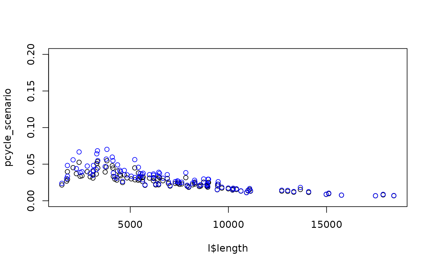
Cycling uptake
--
Dose/response modelling: about cycling in response to distance, hilliness and other factors. Source: pct R package website
background-image: url(https://user-images.githubusercontent.com/1825120/96583573-d3c1eb00-12d4-11eb-88b8-ca78087b63f7.png)
Live demo of the PCT for Bristol
See https://www.pct.bike/
.pull-left[
Uses of the PCT
- Visioning
- Planning strategic cycle networks
- Identifying corridors with high latent demand
Uses that were not initially planned
- Pop-up cycleway planning
- LTN planning?
]
--
.pull-right[
What it cannot do
- Junction design
- Exact route plan (PCT results are based on 'fastest route')
- Public-transport integration
- Other trip purposes beyond single stage journeys cycling to work and school
- Planning for future developments
]
--
For further info, see the training materials at itsleeds.github.io
Many use cases on the PCT website: pct.bike/manual.html
- Case studies of over a dozen areas, including Greater Manchester and Herefordshire in the manual
Estimating health benefits of cycling uptake with the PCT
- The PCT uses a modified version of the HEAT methodology to calculate health benefits of scenarios of change
- Based on the DfT's TAG methodology
- The scenarios are what if scenarios not forecasts
- See the PCT manual for further information: pct.bike/manual.html
- See the DfT's AMAT tool also

From evidence to network plans
Plans from Leeds City Council responding to national guidance and funding for 'pop-up' cycleways (image credit: Leeds City Council):
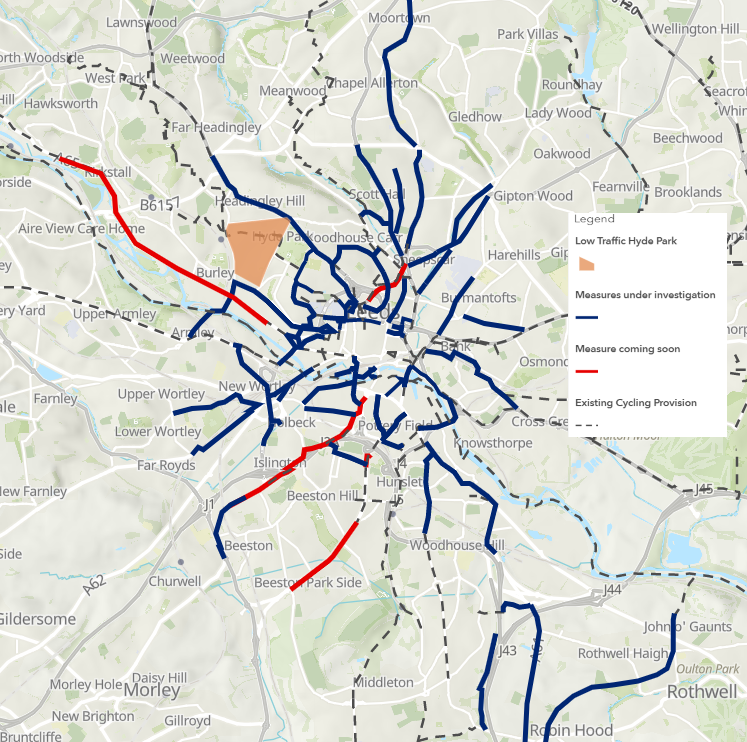
background-image: url(https://raw.githubusercontent.com/cyipt/popupCycleways/master/figures/results-top-leeds.png)
The Rapid tool - see cyipt.bike/rapid
- Live demo by Joey Talbot
The PCT Advanced Workshop
12th November, 2pm, online

The team
Robin Lovelace
- Geographer by Training
- Associate Professor in Transport Data Science, Institute for Transport Studies, University of Leeds
- Lead Developer of the Propensity to Cycle Tool
- R developer and teacher, author of open source books Efficient R Programming and Gecomputation with R
--
Joey Talbot
- Experienced data scientist
- Policy and planning knowledge through role in Transport for New Homes
Rosa Félix
- Transport Engineer by training
- Working on cycling potential and infrastructure prioritisation
How about you?
.pull-left[

]
--
.pull-right[

]
Overview of workshop
Part 1: how the Propensity to Cycle Tool works + demo: 'I do'
- Introductions (14:00 - 14:15)
- Walk through of
test-setup.R (14:15 - 14:40)
- Demonstration of cycling potential in a new context (14:40 - 14:45)
- Questions, break and debugging the test code in breakout rooms (14:45 - 15:00)
- Room 1: technical questions and debugging code (Joey)
- Room 2: methodological questions about the PCT (Robin)
- Room 3: applying the PCT in new contexts (Rosa)
- Room 4: networking
--
Part 2: Co-coding session: getting started with transport data in R: 'we do'
- Working through the code in
pct_training.R (15:00 - 15:30)
- Breakout rooms 2 and 3 open for people who have questions
- Live demo: overlaying PCT data with data from the Rapid tool and OSM (15:30 - 15:45)
☕☕☕ 15 minute break ☕☕☕
Workshop overview - Part III
Part 3: using PCT data for local transport planning: 'you do'
-
Getting set-up with RStudio and input data (16:00 - 16:15, Robin)
-
Break-out rooms (16:15 - 17:00)
- Getting and visualising PCT data (e.g.
get_pct_rnet)
- Running the PCT for new areas
-
Advanced topics (different routing, uptake and route network summary methods - developments in stplanr)
-
Presentation of work and next steps (17:00 - 17:15)
- Networking and 'ideas with beers' 🍻🍻🍻 (17:20 - 18:00)
library(leaflet)
l = stplanr::geo_code("Institute for Transport Studies, University of Leeds")
leaflet() %>%
  addProviderTiles(provider = providers$OpenStreetMap.BlackAndWhite) %>%
  addMarkers(lng = l[1], lat = l[2])
Learning outcomes
- Understand the data and code underlying the PCT
- Download data from the PCT at various geographic levels
- Use R as a tool for data analysis to support evidence-based planning
--
It's about free and open source software for a sustainable future r emojifont::emoji("rocket")

background-image: url(https://media.giphy.com/media/YlQQYUIEAZ76o/giphy.gif)
Coding
Ideal:
od_test$perc_cycle = round(od_test$bicycle / od_test$all) * 100
l = od_to_sf(od_test, od_data_centroids)
r = stplanr::route(l = l, route_fun = journey)
rnet = overline(r, "bicycle")
--

Reality
Key stages of PCT approach
- Reproducible, open, scripted, enabling modifications, e.g.:
- Find short routes in which more people drive than cycle
--
- Stage 1: get data
# Aim: get top 1000 lines in repo
library(dplyr)
library(sf)
desire_lines_all = pct::get_pct_lines(region = "isle-of-wight")
desire_lines = desire_lines_all %>%
  top_n(1000, all)
write_sf(desire_lines, "desire_lines.geojson")
piggyback::pb_upload("desire_lines.geojson")
# Set-up, after installing pct and checking out www.pct.bike:
library(dplyr)
library(sf)
desire_lines_all = pct::get_pct_lines(region = "isle-of-wight") %>%
  top_n(n = 1000, wt = all)
Stage II: Subset data of interest
- Interested only in major lines
library(sf)
desire_lines = desire_lines_all %>%
  filter(all > 50) %>%
  select(geo_code1, geo_code2, all, bicycle, foot, car_driver, rf_dist_km)
plot(desire_lines)
Stage III: Visualisation
.pull-left[
plot(desire_lines)
]
.pull-right[
]
library(tmap)
tmap_mode("view")
tm_shape(desire_lines) +
  tm_lines("all", scale = 9) +
  tm_basemap(server = leaflet::providers$OpenStreetMap)
Stage IV: Origin-destination data analysis
-
Now we have data in our computer, and verified it works, we can use it
-
Which places are most car dependent?
car_dependent_routes = desire_lines %>%
  mutate(percent_drive = car_driver / all * 100) %>%
  filter(rf_dist_km < 3 & rf_dist_km > 1)
- Get routes
routes = stplanr::line2route(car_dependent_routes)
car_dependent_routes$geometry = routes$geometry
Other topics
Transport software - which do you use?
u = "https://github.com/ITSLeeds/TDS/raw/master/transport-software.csv"
tms = readr::read_csv(u)[1:5]
tms = dplyr::arrange(tms, dplyr::desc(Citations))
knitr::kable(tms, booktabs = TRUE, caption = "Sample of transport modelling software in use by practitioners. Note: citation counts based on searches for company/developer name, the product name and 'transport'. Data source: Google Scholar searches, October 2018.", format = "html")
Data science and the tidyverse
- Inspired by Introduction to data science with R (available free online)
r Citep(my_bib, "grolemund_r_2016", .opts = list(cite.style = "authoryear"))
knitr::include_graphics("https://d33wubrfki0l68.cloudfront.net/b88ef926a004b0fce72b2526b0b5c4413666a4cb/24a30/cover.png")
A geographic perspective
-
See https://github.com/ITSLeeds/TDS/blob/master/catalogue.md
-
Paper on the stplanr paper for transport planning (available online) r Citep(my_bib, "lovelace_stplanr:_2018", .opts = list(cite.style = "authoryear"))
- Introductory and advanced content on geographic data in R, especially the transport chapter (available free online)
r Citep(my_bib, "lovelace_geocomputation_2019", .opts = list(cite.style = "authoryear"))
- Paper on analysing OSM data in Python
r Citep(my_bib, "boeing_osmnx_2017", .opts = list(cite.style = "authoryear")) (available online)
Getting support
--
With open source software, the world is your support network!
--
- Recent example: https://stackoverflow.com/questions/57235601/
--
-
gis.stackexchange.com has 21,314 questions
-
r-sig-geo has 1000s of posts
-
RStudio's Discourse community has 65,000+ posts already!
--
-
No transport equivalent (e.g. earthscience.stackexchange.com is in beta)
-
Potential for a Discourse forum or similar: transport is not (just) GIS
References
PrintBibliography(my_bib)
# RefManageR::WriteBib(my_bib, "refs-geostat.bib")
Try the pct package in your browser
Any scripts or data that you put into this service are public.
pct documentation built on April 4, 2025, 4:12 a.m.
R Package Documentation
Browse R Packages
We want your feedback!
Note that we can't provide technical support on individual packages. You should contact the package authors for that.
# get citations refs = RefManageR::ReadZotero(group = "418217", .params = list(collection = "JFR868KJ", limit = 100)) refs_df = as.data.frame(refs) # View(refs_df) # citr::insert_citation(bib_file = "vignettes/refs_training.bib") RefManageR::WriteBib(refs, "refs.bib") # citr::tidy_bib_file(rmd_file = "vignettes/pct_training.Rmd", messy_bibliography = "vignettes/refs_training.bib") options(htmltools.dir.version = FALSE) knitr::opts_chunk$set(message = FALSE) library(RefManageR) BibOptions(check.entries = FALSE, bib.style = "authoryear", cite.style = 'alphabetic', style = "markdown", first.inits = FALSE, hyperlink = FALSE, dashed = FALSE) my_bib = refs
library(RefManageR) my_bib = RefManageR::ReadBib("refs.bib")
# publish results online cp -Rv inst/rmd/pct-slides* ~/saferactive/site/static/slides/ cp -Rv inst/rmd/libs ~/saferactive/site/static/slides/ cd ~/saferactive/site git add -A git status git commit -am 'Update slides' git push cd -
Intro + agenda
This workshop will provide an overview of the PCT for advanced users, including:
- transport planners with experience of evidence-based prioritisation
- researchers with experience of using origin-destination, route and route network level data
- programmers, developers and others wanting to extend PCT methods for the public benefit
--
The workshop will be broken into three main parts:
Part 1: how the Propensity to Cycle Tool works + demo: 'I do' (14:00 - 15:00)
Part 2: Co-coding session: 'we do' (15:00 - 15:45)
☕☕☕ 15 minute break ☕☕☕
Part 3: using PCT data for your needs: 'you do' (16:00 - 17:00)
- Presentation of work and next steps (17:00 - 17:15)
- Networking and 'ideas with beers' 🍻🍻🍻 (17:20 - 18:00)
Description:
In this workshop you will take a deep dive into the Propensity to Cycle Tool (PCT). Beginner and intermediate PCT events focus on using the PCT via the web application hosted at www.pct.bike and the data provided by the PCT in QGIS but the focus here is on analysing cycling potential in the open source statistical programming language R. The majority of the PCT was built on R, which is a powerful object-orientated programming language with a focus on statistical modelling, visualisation and geographic analysis. The workshop will show how the code underlying the PCT works, how the underlying data can be accessed for reproducible analysis, and how the methods can be used to generate new scenarios of cycling uptake.
Preparation
If you are inexperienced with R you should prepare by
- Essential: taking an online course such as the free 'Introduction to R' course provided by DataCamp
- Essential: ensuring you have installed up-to-date versions of R (R 4.0.0 or greater), RStudio (1.2 or greater) and the pct R package (0.6.0) on your computer
- Essential: test your computer set up by running the R code here github.com/ITSLeeds/pct/blob/master/inst/test-setup.R - you should make a note of the result of this final commented-out command:
round(mean(rnet_potential$Potential)) - Highly recommended: working through and reproducing results in Chapter 12 onwards of the open source book Geocomputation with R (see geocompr.robinlovelace.net/transport.html)
If you are new to R but have not completed the above tasks you may be unable to follow the second and third sections of the workshop outlined in the agenda below.
Prerequisites
See here for a guide on installing R and RStudio for transport data research. To get the access code for the tutorial, you will need to first work through the code shown here: https://github.com/ITSLeeds/pct/blob/master/inst/test-setup.R After you have run the code, running the following line should give you a number that will give you the access code for the course:
round(mean(rnet_potential$Potential))
Save that 3 digit number, it will allow access to the workshop. If you have any issues with your computer set-up, please ask a question here (you will need to sign-up for a GitHub account if you have not already done so): https://github.com/ITSLeeds/pct/issues/67
background-image: url(https://media.giphy.com/media/YlQQYUIEAZ76o/giphy.gif) background-size: cover class: center, middle
How the PCT works
The first prototype of the PCT
-
1st prototype: Hackathon at ODI Leeds in February 2015
-
We identifying key routes and mapped them
-
For description of aims, see Lovelace et al. (2017)
knitr::include_graphics("https://raw.githubusercontent.com/npct/pct-team/master/figures/early.png")
- Launched in 2017 with the Cycling and Walking Investment Strategy (CWIS)
Photo: demo of the PCT to Secretary of State for Transport (March 2017)
The PCT in 2020
- Now the go-to tool for strategic cycle network planning in England and Wales, used by most local authorities with cycling plans (source).
.pull-left[
Geographic levels in the PCT
- Generate and analyse route networks for transport planning with reference to:
- Zones
- Origin-destination (OD) data
- Geographic desire lines
- Route allocation using different routing services
- Route network generation and analysis ]
.pull-right[
See these levels at www.pct.bike
]
Let's look at zones
qtm(od_data_zones_min)
MSOA vs LSOA zones (MSOA zones ~5 times bigger)
# not the best example # knitr::include_graphics("https://user-images.githubusercontent.com/1825120/96573136-a1f55800-12c5-11eb-8921-c9938cd9e929.gif") knitr::include_graphics(c( "https://user-images.githubusercontent.com/1825120/96583573-d3c1eb00-12d4-11eb-88b8-ca78087b63f7.png", "https://user-images.githubusercontent.com/1825120/96583629-eb00d880-12d4-11eb-9211-d015e2991267.png" )) # 32844 / 6791
- MSOA areas have a population of 5-15k
- LSOAs have a population of 1-3k
- Route network data in PCT data based on LSOA data
- MSOAs can be useful for identifying key desire lines
- See ons.gov.uk for details
OD data
library(tmap) library(od) tmap_mode("plot") od_test = od::od_data_df od_test$id = 1:nrow(od_test) od_test$perc_cycle = round(od_test$bicycle / od_test$all, 3) * 100 knitr::kable(od_test, caption = "Origin-destination data. Open MSOA-MSOA commute data from the 2011 census, accessed using the R package pct.")
Desire lines
l = od_to_sf(od_test, od_data_centroids) l = dplyr::select(l, id, foot, bicycle, car_driver, perc_cycle) p = od_data_centroids p = p[l, ] tm_shape(l) + tm_lines("perc_cycle", palette = "viridis", lwd = "car_driver", legend.lwd.show = FALSE, scale = 9, alpha = 0.5) + tm_text("id") + tm_shape(p) + tm_text("geo_code")
Routes
library(cyclestreets) r = stplanr::route(l = l, route_fun = journey) saveRDS(r, "routes_od_data_df_df.Rds") piggyback::pb_upload("routes_od_data_df_df.Rds") piggyback::pb_download_url("routes_od_data_df_df.Rds") file.remove("routes_od_data_df_df.Rds")
tm_shape(r) + tm_lines("perc_cycle", palette = "viridis", lwd = "car_driver", legend.lwd.show = FALSE, scale = 9, alpha = 0.5) + tm_shape(p) + tm_text("geo_code")
Route networks
u = "https://github.com/ITSLeeds/pct/releases/download/0.5.0/routes_od_data_df_df.Rds" f = basename(u) if(!file.exists(f)){ download.file(u, f) } r = readRDS(f)
rnet = stplanr::overline(r, "bicycle") plot(rnet, lwd = rnet$bicycle / 10)
Cycling uptake
--
Dose/response modelling: about cycling in response to distance, hilliness and other factors. Source: pct R package website
background-image: url(https://user-images.githubusercontent.com/1825120/96583573-d3c1eb00-12d4-11eb-88b8-ca78087b63f7.png)
Live demo of the PCT for Bristol
See https://www.pct.bike/
.pull-left[
Uses of the PCT
- Visioning
- Planning strategic cycle networks
- Identifying corridors with high latent demand
Uses that were not initially planned
- Pop-up cycleway planning
- LTN planning?
]
--
.pull-right[
What it cannot do
- Junction design
- Exact route plan (PCT results are based on 'fastest route')
- Public-transport integration
- Other trip purposes beyond single stage journeys cycling to work and school
- Planning for future developments
]
--
For further info, see the training materials at itsleeds.github.io
Many use cases on the PCT website: pct.bike/manual.html
- Case studies of over a dozen areas, including Greater Manchester and Herefordshire in the manual
Estimating health benefits of cycling uptake with the PCT
- The PCT uses a modified version of the HEAT methodology to calculate health benefits of scenarios of change
- Based on the DfT's TAG methodology
- The scenarios are what if scenarios not forecasts
- See the PCT manual for further information: pct.bike/manual.html
- See the DfT's AMAT tool also
From evidence to network plans
Plans from Leeds City Council responding to national guidance and funding for 'pop-up' cycleways (image credit: Leeds City Council):
background-image: url(https://raw.githubusercontent.com/cyipt/popupCycleways/master/figures/results-top-leeds.png)
The Rapid tool - see cyipt.bike/rapid
- Live demo by Joey Talbot
The PCT Advanced Workshop
12th November, 2pm, online
The team
Robin Lovelace
- Geographer by Training
- Associate Professor in Transport Data Science, Institute for Transport Studies, University of Leeds
- Lead Developer of the Propensity to Cycle Tool
- R developer and teacher, author of open source books Efficient R Programming and Gecomputation with R
--
Joey Talbot
- Experienced data scientist
- Policy and planning knowledge through role in Transport for New Homes
Rosa Félix
- Transport Engineer by training
- Working on cycling potential and infrastructure prioritisation
How about you?
.pull-left[
]
--
.pull-right[
]
Overview of workshop
Part 1: how the Propensity to Cycle Tool works + demo: 'I do'
- Introductions (14:00 - 14:15)
- Walk through of
test-setup.R(14:15 - 14:40) - Demonstration of cycling potential in a new context (14:40 - 14:45)
- Questions, break and debugging the test code in breakout rooms (14:45 - 15:00)
- Room 1: technical questions and debugging code (Joey)
- Room 2: methodological questions about the PCT (Robin)
- Room 3: applying the PCT in new contexts (Rosa)
- Room 4: networking
--
Part 2: Co-coding session: getting started with transport data in R: 'we do'
- Working through the code in
pct_training.R(15:00 - 15:30) - Breakout rooms 2 and 3 open for people who have questions
- Live demo: overlaying PCT data with data from the Rapid tool and OSM (15:30 - 15:45)
☕☕☕ 15 minute break ☕☕☕
Workshop overview - Part III
Part 3: using PCT data for local transport planning: 'you do'
-
Getting set-up with RStudio and input data (16:00 - 16:15, Robin)
-
Break-out rooms (16:15 - 17:00)
- Getting and visualising PCT data (e.g.
get_pct_rnet) - Running the PCT for new areas
-
Advanced topics (different routing, uptake and route network summary methods - developments in stplanr)
-
Presentation of work and next steps (17:00 - 17:15)
- Networking and 'ideas with beers' 🍻🍻🍻 (17:20 - 18:00)
library(leaflet) l = stplanr::geo_code("Institute for Transport Studies, University of Leeds") leaflet() %>% addProviderTiles(provider = providers$OpenStreetMap.BlackAndWhite) %>% addMarkers(lng = l[1], lat = l[2])
Learning outcomes
- Understand the data and code underlying the PCT
- Download data from the PCT at various geographic levels
- Use R as a tool for data analysis to support evidence-based planning
--
It's about free and open source software for a sustainable future r emojifont::emoji("rocket")
background-image: url(https://media.giphy.com/media/YlQQYUIEAZ76o/giphy.gif)
Coding
Ideal:
od_test$perc_cycle = round(od_test$bicycle / od_test$all) * 100 l = od_to_sf(od_test, od_data_centroids) r = stplanr::route(l = l, route_fun = journey) rnet = overline(r, "bicycle")
--
Reality
Key stages of PCT approach
- Reproducible, open, scripted, enabling modifications, e.g.:
- Find short routes in which more people drive than cycle
--
- Stage 1: get data
# Aim: get top 1000 lines in repo library(dplyr) library(sf) desire_lines_all = pct::get_pct_lines(region = "isle-of-wight") desire_lines = desire_lines_all %>% top_n(1000, all) write_sf(desire_lines, "desire_lines.geojson") piggyback::pb_upload("desire_lines.geojson")
# Set-up, after installing pct and checking out www.pct.bike: library(dplyr) library(sf) desire_lines_all = pct::get_pct_lines(region = "isle-of-wight") %>% top_n(n = 1000, wt = all)
Stage II: Subset data of interest
- Interested only in major lines
library(sf) desire_lines = desire_lines_all %>% filter(all > 50) %>% select(geo_code1, geo_code2, all, bicycle, foot, car_driver, rf_dist_km) plot(desire_lines)
Stage III: Visualisation
.pull-left[ plot(desire_lines) ] .pull-right[ ]
library(tmap) tmap_mode("view") tm_shape(desire_lines) + tm_lines("all", scale = 9) + tm_basemap(server = leaflet::providers$OpenStreetMap)
Stage IV: Origin-destination data analysis
-
Now we have data in our computer, and verified it works, we can use it
-
Which places are most car dependent?
car_dependent_routes = desire_lines %>% mutate(percent_drive = car_driver / all * 100) %>% filter(rf_dist_km < 3 & rf_dist_km > 1)
- Get routes
routes = stplanr::line2route(car_dependent_routes) car_dependent_routes$geometry = routes$geometry
Other topics
Transport software - which do you use?
u = "https://github.com/ITSLeeds/TDS/raw/master/transport-software.csv" tms = readr::read_csv(u)[1:5] tms = dplyr::arrange(tms, dplyr::desc(Citations)) knitr::kable(tms, booktabs = TRUE, caption = "Sample of transport modelling software in use by practitioners. Note: citation counts based on searches for company/developer name, the product name and 'transport'. Data source: Google Scholar searches, October 2018.", format = "html")
Data science and the tidyverse
- Inspired by Introduction to data science with R (available free online)
r Citep(my_bib, "grolemund_r_2016", .opts = list(cite.style = "authoryear"))
knitr::include_graphics("https://d33wubrfki0l68.cloudfront.net/b88ef926a004b0fce72b2526b0b5c4413666a4cb/24a30/cover.png")
A geographic perspective
-
See https://github.com/ITSLeeds/TDS/blob/master/catalogue.md
-
Paper on the stplanr paper for transport planning (available online)
r Citep(my_bib, "lovelace_stplanr:_2018", .opts = list(cite.style = "authoryear")) - Introductory and advanced content on geographic data in R, especially the transport chapter (available free online)
r Citep(my_bib, "lovelace_geocomputation_2019", .opts = list(cite.style = "authoryear")) - Paper on analysing OSM data in Python
r Citep(my_bib, "boeing_osmnx_2017", .opts = list(cite.style = "authoryear"))(available online)
Getting support
--
With open source software, the world is your support network!
--
- Recent example: https://stackoverflow.com/questions/57235601/
--
-
gis.stackexchange.com has 21,314 questions
-
r-sig-geo has 1000s of posts
-
RStudio's Discourse community has 65,000+ posts already!
--
-
No transport equivalent (e.g. earthscience.stackexchange.com is in beta)
-
Potential for a Discourse forum or similar: transport is not (just) GIS
References
PrintBibliography(my_bib) # RefManageR::WriteBib(my_bib, "refs-geostat.bib")
Try the pct package in your browser
Any scripts or data that you put into this service are public.
R Package Documentation
Browse R Packages
We want your feedback!
Note that we can't provide technical support on individual packages. You should contact the package authors for that.
Embedding an R snippet on your website
Add the following code to your website.
For more information on customizing the embed code, read Embedding Snippets.