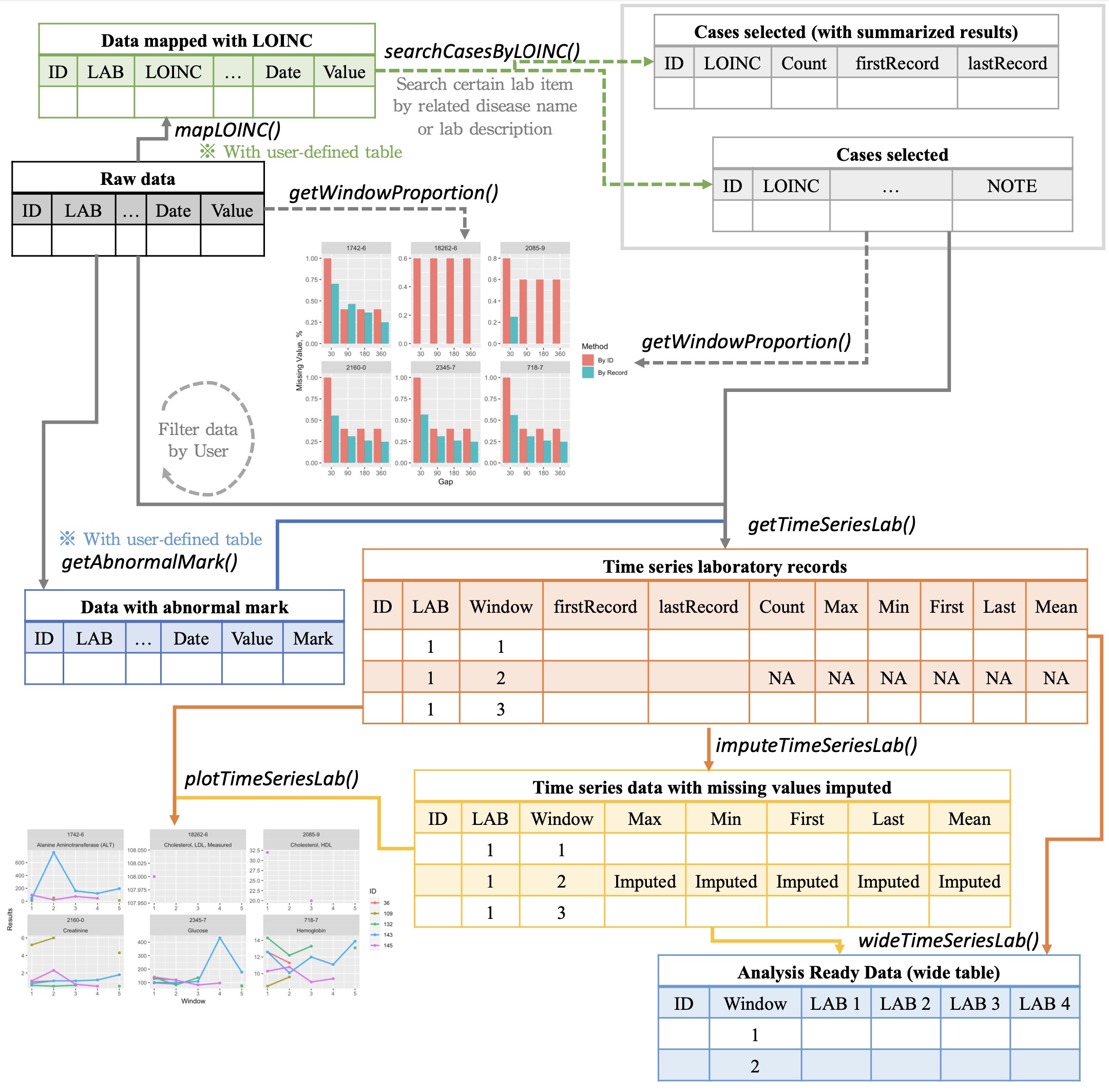
In DHLab-TSENG/lab: a package for EHR laboratory data
knitr::opts_chunk$set(echo = TRUE)
For full references, please refer to: https://dhlab-tseng.github.io/lab/index.html

I. Introduction
The proposed open-source lab package is a software tool that help users to explore and process laboratory data in electronic health records (EHRs). With the lab package, researchers can easily map local laboratory codes to the universal standard, mark abnormal results, summarize data using descriptive statistics, impute missing values, and generate analysis ready data.
Feature
- Data Mapping Standardize and manipulate data with Logical Observation Identifiers Names and Codes (LOINC), a common terminology for laboratory and clinical observations.
- Time Series Analysis Separate lab test results into multiple consecutive non-overlapped time windows
- Value Imputation Impute value to replace missing data
- Wide Format Generation Transform longitudinal data into wide format to generate analysis ready data
Development version
# install.packages("remotes")
remotes::install_github("DHLab-TSENG/lab")
knitr::opts_chunk$set(collapse = T, comment = "#>")
options(tibble.print_min = 4L, tibble.print_max = 4L)
#remotes::install_github("DHLab-TSENG/lab")
library(lab)
Overview

Usage
# install.packages("remotes")
remotes::install_github("DHLab-TSENG/lab")
library(lab)
Dataset
The sample data includes 1,744 lab records containing 7 different lab items tested by 5 patients from MIMIC-III database.
head(labSample)
I. Data Mapping
If LOINC is not the default terminology, users are recommended to map local lab item with LOINC by providing mapping table.
First, user shall prepare a mapping table with local codes and LOINC codes.
head(mapSample)
loincSample <- mapLOINC(labData = labSample, labItemColName = ITEMID, mappingTable = mapSample)

head(loincSample)
Once a user map lab test codes with LOINC, ranges can be used to mark abnormal results, and related names can be used to search related lab test codes by other common names of a lab test.
loincMarkedSample <- getAbnormalMark(labData = loincSample,
                                     idColName = SUBJECT_ID,
                                     labItemColName = LOINC,
                                     valueColName = VALUENUM,
                                     genderColName = GENDER,
                                     genderTable = patientSample,
                                     referenceTable = refLOINC)
head(loincMarkedSample)
caseCreatinine <- searchCasesByLOINC(labData = loincSample,
                                     idColName = SUBJECT_ID,
                                     loincColName = LOINC,
                                     dateColName = CHARTTIME,
                                     condition = "Creatinine",
                                     isSummary = TRUE)

head(caseCreatinine)
II. Time Series Analysis
lab package allows users to separate lab test results into multiple consecutive non-overlapped time windows.
The index date of time windows can be the first or last event occurred for individuals, or a specific date for all patients.
To help users find suitable window size (e.g., 30 days or 180 days, to name but a few), a plot function is provided to visualize how frequent the patients did each lab test.
windowProportion <- plotWindowProportion(labData = loincSample,
                                         idColName = SUBJECT_ID,
                                         labItemColName = LOINC,
                                         dateColName = CHARTTIME,
                                         indexDate = first,
                                         gapDate = c(30, 90, 180, 360),
                                         studyPeriodStartDays=0,
                                         studyPeriodEndDays=360)

print(windowProportion$graph)

head(windowProportion$missingData)
After the index date and window size are decided, the descriptive statistics information, including total test times within a window, maximum test value, minimum test value, test values average, and the record nearest to the index date, are shown.
timeSeriesData <- getTimeSeriesLab(labData = loincSample,
                                   idColName = SUBJECT_ID,
                                   labItemColName = LOINC + LABEL,
                                   dateColName = CHARTTIME,
                                   valueColName = VALUENUM,
                                   indexDate = first,
                                   gapDate = 30,
                                   completeWindows = TRUE)
head(timeSeriesData)
Also, a line chart plotting function is available to do long-term follow-up. Visualization is helpful for detecting data trends. Additionally, “L” and “H” will be used as legendary icon if abnormal values are marked.
timeSeriesPlot <- plotTimeSeriesLab(labData = timeSeriesData,
                                    idColName = ID,
                                    labItemColName = LOINC + LABEL,
                                    timeMarkColName = Window,
                                    valueColName = Nearest,
                                    timeStart = 1,
                                    timeEnd  = 5,
                                    abnormalMarkColName = NULL)

plot(timeSeriesPlot)
III. Imputation
Imputation function can be executed to replace missing data.
fullTimeSeriesData <- imputeTimeSeriesLab(labData = timeSeriesData,
                                          idColName = ID,
                                          labItemColName = LOINC + LABEL,
                                          windowColName = Window,
                                          valueColName = Mean & Nearest,
                                          impMethod = NOCB,
                                          imputeOverallMean = FALSE)
fullTimeSeriesData[timeSeriesData$ID==36&
                     timeSeriesData$LOINC=="2160-0"]
IV. Wide Format Generation
Then, a function be used to transform longitudinal data into wide format to generate analysis ready data.
wideTimeSeriesData <- wideTimeSeriesLab(labData = fullTimeSeriesData,
                                        idColName = ID,
                                        labItemColName = LOINC + LABEL,
                                        windowColName = Window,
                                        valueColName = Nearest)
head(wideTimeSeriesData)
V. Machine Learning Application
Wide format date is commonly utilized in machine learning methods. In this package, we provide an k-nearest neighbors (kNN) imputation function enabling users to impute missing values by machine learning technique with wide format data.
wideTimeSeriesData <- wideTimeSeriesLab(labData = timeSeriesData,
                                        idColName = ID,
                                        labItemColName = LOINC + LABEL,
                                        windowColName = Window,
                                        valueColName = Nearest)

knnImputedData <- imputeKNN(labData = wideTimeSeriesData,
                            idColName = ID + Window,
                            k = 1)

head(knnImputedData)
DHLab-TSENG/lab documentation built on Sept. 1, 2023, 9:03 p.m.
knitr::opts_chunk$set(echo = TRUE)
For full references, please refer to: https://dhlab-tseng.github.io/lab/index.html

I. Introduction
The proposed open-source lab package is a software tool that help users to explore and process laboratory data in electronic health records (EHRs). With the lab package, researchers can easily map local laboratory codes to the universal standard, mark abnormal results, summarize data using descriptive statistics, impute missing values, and generate analysis ready data.
Feature
- Data Mapping Standardize and manipulate data with Logical Observation Identifiers Names and Codes (LOINC), a common terminology for laboratory and clinical observations.
- Time Series Analysis Separate lab test results into multiple consecutive non-overlapped time windows
- Value Imputation Impute value to replace missing data
- Wide Format Generation Transform longitudinal data into wide format to generate analysis ready data
Development version
# install.packages("remotes") remotes::install_github("DHLab-TSENG/lab")
knitr::opts_chunk$set(collapse = T, comment = "#>") options(tibble.print_min = 4L, tibble.print_max = 4L) #remotes::install_github("DHLab-TSENG/lab") library(lab)
Overview

Usage
# install.packages("remotes") remotes::install_github("DHLab-TSENG/lab") library(lab)
Dataset
The sample data includes 1,744 lab records containing 7 different lab items tested by 5 patients from MIMIC-III database.
head(labSample)
I. Data Mapping
If LOINC is not the default terminology, users are recommended to map local lab item with LOINC by providing mapping table.
First, user shall prepare a mapping table with local codes and LOINC codes.
head(mapSample)
loincSample <- mapLOINC(labData = labSample, labItemColName = ITEMID, mappingTable = mapSample) head(loincSample)
Once a user map lab test codes with LOINC, ranges can be used to mark abnormal results, and related names can be used to search related lab test codes by other common names of a lab test.
loincMarkedSample <- getAbnormalMark(labData = loincSample, idColName = SUBJECT_ID, labItemColName = LOINC, valueColName = VALUENUM, genderColName = GENDER, genderTable = patientSample, referenceTable = refLOINC) head(loincMarkedSample)
caseCreatinine <- searchCasesByLOINC(labData = loincSample, idColName = SUBJECT_ID, loincColName = LOINC, dateColName = CHARTTIME, condition = "Creatinine", isSummary = TRUE) head(caseCreatinine)
II. Time Series Analysis
lab package allows users to separate lab test results into multiple consecutive non-overlapped time windows. The index date of time windows can be the first or last event occurred for individuals, or a specific date for all patients. To help users find suitable window size (e.g., 30 days or 180 days, to name but a few), a plot function is provided to visualize how frequent the patients did each lab test.
windowProportion <- plotWindowProportion(labData = loincSample, idColName = SUBJECT_ID, labItemColName = LOINC, dateColName = CHARTTIME, indexDate = first, gapDate = c(30, 90, 180, 360), studyPeriodStartDays=0, studyPeriodEndDays=360) print(windowProportion$graph) head(windowProportion$missingData)
After the index date and window size are decided, the descriptive statistics information, including total test times within a window, maximum test value, minimum test value, test values average, and the record nearest to the index date, are shown.
timeSeriesData <- getTimeSeriesLab(labData = loincSample, idColName = SUBJECT_ID, labItemColName = LOINC + LABEL, dateColName = CHARTTIME, valueColName = VALUENUM, indexDate = first, gapDate = 30, completeWindows = TRUE) head(timeSeriesData)
Also, a line chart plotting function is available to do long-term follow-up. Visualization is helpful for detecting data trends. Additionally, “L” and “H” will be used as legendary icon if abnormal values are marked.
timeSeriesPlot <- plotTimeSeriesLab(labData = timeSeriesData, idColName = ID, labItemColName = LOINC + LABEL, timeMarkColName = Window, valueColName = Nearest, timeStart = 1, timeEnd = 5, abnormalMarkColName = NULL) plot(timeSeriesPlot)
III. Imputation
Imputation function can be executed to replace missing data.
fullTimeSeriesData <- imputeTimeSeriesLab(labData = timeSeriesData, idColName = ID, labItemColName = LOINC + LABEL, windowColName = Window, valueColName = Mean & Nearest, impMethod = NOCB, imputeOverallMean = FALSE) fullTimeSeriesData[timeSeriesData$ID==36& timeSeriesData$LOINC=="2160-0"]
IV. Wide Format Generation
Then, a function be used to transform longitudinal data into wide format to generate analysis ready data.
wideTimeSeriesData <- wideTimeSeriesLab(labData = fullTimeSeriesData, idColName = ID, labItemColName = LOINC + LABEL, windowColName = Window, valueColName = Nearest) head(wideTimeSeriesData)
V. Machine Learning Application
Wide format date is commonly utilized in machine learning methods. In this package, we provide an k-nearest neighbors (kNN) imputation function enabling users to impute missing values by machine learning technique with wide format data.
wideTimeSeriesData <- wideTimeSeriesLab(labData = timeSeriesData, idColName = ID, labItemColName = LOINC + LABEL, windowColName = Window, valueColName = Nearest) knnImputedData <- imputeKNN(labData = wideTimeSeriesData, idColName = ID + Window, k = 1) head(knnImputedData)
Add the following code to your website.
For more information on customizing the embed code, read Embedding Snippets.
