In LieberInstitute/TREG: Tools for finding Total RNA Expression Genes in single nucleus RNA-seq data

knitr::opts_chunk$set(
    collapse = TRUE,
    comment = "#>"
)

## For links
library("BiocStyle")

## Track time spent on making the vignette
startTime <- Sys.time()

# Bib setup
library("RefManageR")

## Write bibliography information
bib <- c(
    R = citation(),
    BiocFileCache = citation("BiocFileCache")[1],
    BiocStyle = citation("BiocStyle")[1],
    dplyr = citation("dplyr")[1],
    ggplot2 = citation("ggplot2")[1],
    knitr = citation("knitr")[1],
    Matrix = citation("Matrix")[1],
    pheatmap = citation("pheatmap")[1],
    purrr = citation("purrr")[1],
    rafalib = citation("rafalib")[1],
    RefManageR = citation("RefManageR")[1],
    rmarkdown = citation("rmarkdown")[1],
    sessioninfo = citation("sessioninfo")[1],
    SummarizedExperiment = citation("SummarizedExperiment")[1],
    testthat = citation("testthat")[1],
    tibble = citation("tibble")[1],
    tidyr = citation("tidyr")[1],
    tran2021 = RefManageR::BibEntry(
        bibtype = "Article",
        key = "tran2021",
        author = "Tran, Matthew N. and Maynard, Kristen R. and Spangler, Abby and Huuki, Louise A. and Montgomery, Kelsey D. and Sadashivaiah, Vijay and Tippani, Madhavi and Barry, Brianna K. and Hancock, Dana B. and Hicks, Stephanie C. and Kleinman, Joel E. and Hyde, Thomas M. and Collado-Torres, Leonardo and Jaffe, Andrew E. and Martinowich, Keri",
        title = "Single-nucleus transcriptome analysis reveals cell-type-specific molecular signatures across reward circuitry in the human brain",
        year = 2021, doi = "10.1016/j.neuron.2021.09.001",
        journal = "Neuron"
    ),
    TREG = citation("TREG")[1],
    TREGpaper = citation("TREG")[2]
)

Note: TREG is pronounced as a single word and fully capitalized, unlike Regulatory T cells, which are known as "Tregs" (pronounced "T-regs"). The work described here is unrelated to regulatory T cells.

Basics

Install TREG

R is an open-source statistical environment which can be easily modified to enhance its functionality via packages. r Biocpkg('TREG') is a R package available via Bioconductor. R can be installed on any operating system from CRAN after which you can install r Biocpkg('TREG') by using the following commands in your R session:

if (!requireNamespace("BiocManager", quietly = TRUE)) {
    install.packages("BiocManager")
}

BiocManager::install("TREG")

## Check that you have a valid Bioconductor installation
BiocManager::valid()

Required knowledge

r Biocpkg('TREG') r Citep(bib[['TREG']]) is based on many other packages and in particular in those that have implemented the infrastructure needed for dealing with single cell RNA sequencing data, visualization functions, and interactive data exploration. That is, packages like r Biocpkg('SummarizedExperiment') that allow you to store the data.

If you are asking yourself the question "Where do I start using Bioconductor?" you might be interested in this blog post.

Asking for help

As package developers, we try to explain clearly how to use our packages and in which order to use the functions. But R and Bioconductor have a steep learning curve so it is critical to learn where to ask for help. The blog post quoted above mentions some but we would like to highlight the Bioconductor support site as the main resource for getting help regarding Bioconductor. Other alternatives are available such as creating GitHub issues and tweeting. However, please note that if you want to receive help you should adhere to the posting guidelines. It is particularly critical that you provide a small reproducible example and your session information so package developers can track down the source of the error.

Citing TREG

We hope that r Biocpkg('TREG') will be useful for your research. Please use the following information to cite the package and the research article describing the data provided by r Biocpkg('TREG'). Thank you!

## Citation info
citation("TREG")

Overview

The r Biocpkg('TREG') r Citep(bib[['TREG']]) package was developed for identifying candidate Total RNA Expression Genes (TREGs) for estimating RNA abundance for individual cells in an snFISH experiment by researchers at the Lieber Institute for Brain Development (LIBD) r Citep(bib[['TREGpaper']]).

In this vignette we'll showcase how you can use the R functions provided by r Biocpkg('TREG') r Citep(bib[['TREG']]) with the snRNA-seq dataset that was recently published by our LIBD collaborators r Citep(bib[['tran2021']]).

To get started, please load the r Biocpkg('TREG') package.

library("TREG")

The goal of TREG is to help find candidate Total RNA Expression Genes (TREGs) in single nucleus (or single cell) RNA-seq data.

Why are TREGs useful?

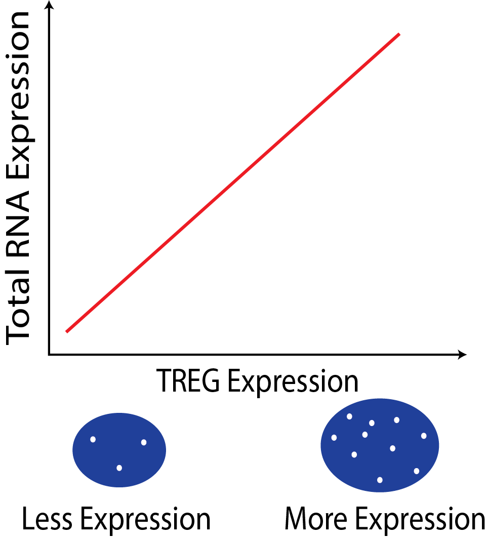
The expression of a TREG is proportional to the the overall RNA expression in a cell. This relationship can be used to estimate total RNA content in cells in assays where only a few genes can be measured, such as single-molecule fluorescent in situ hybridization (smFISH).

In a smFISH experiment the number of TREG puncta can be used to infer the total RNA expression of the cell.

The motivation of this work is to collect data via smFISH in to help build better deconvolution algorithms. But may be many other application for TREGs in experimental design!

{width=50%}

What makes a gene a good TREG?

1. The gene must have non-zero expression in most cells across different tissue and cell types.

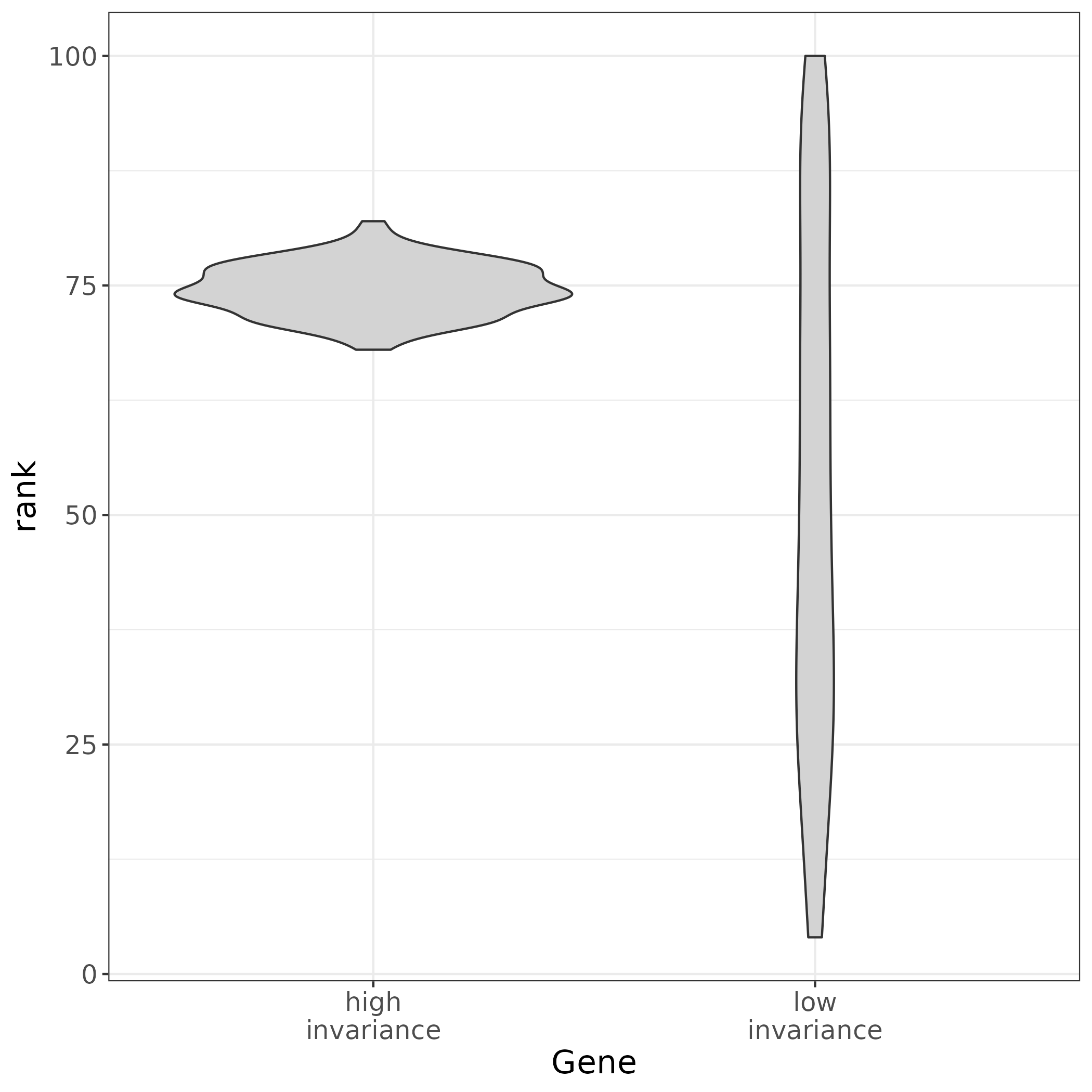
2. A TREG should also be expressed at a constant level in respect to other genes across different cell types or have high rank invariance.

3. Be measurable as a continuous metric in the experimental assay, for example have a dynamic range of puncta when observed in RNAscope. This will need to be considered for the candidate TREGs, and may need to be validated experimentally.

{width=30%}

How to find candidate TREGs with TREG

{width=100%}

1. Filter for low Proportion Zero genes snRNA-seq dataset: This is facilitated with the functions get_prop_zero() and filter_prop_zero() (Equation \@ref(eq:propZero)). snRNA-seq data is notoriously sparse, these functions enrich for genes with more universal expression.

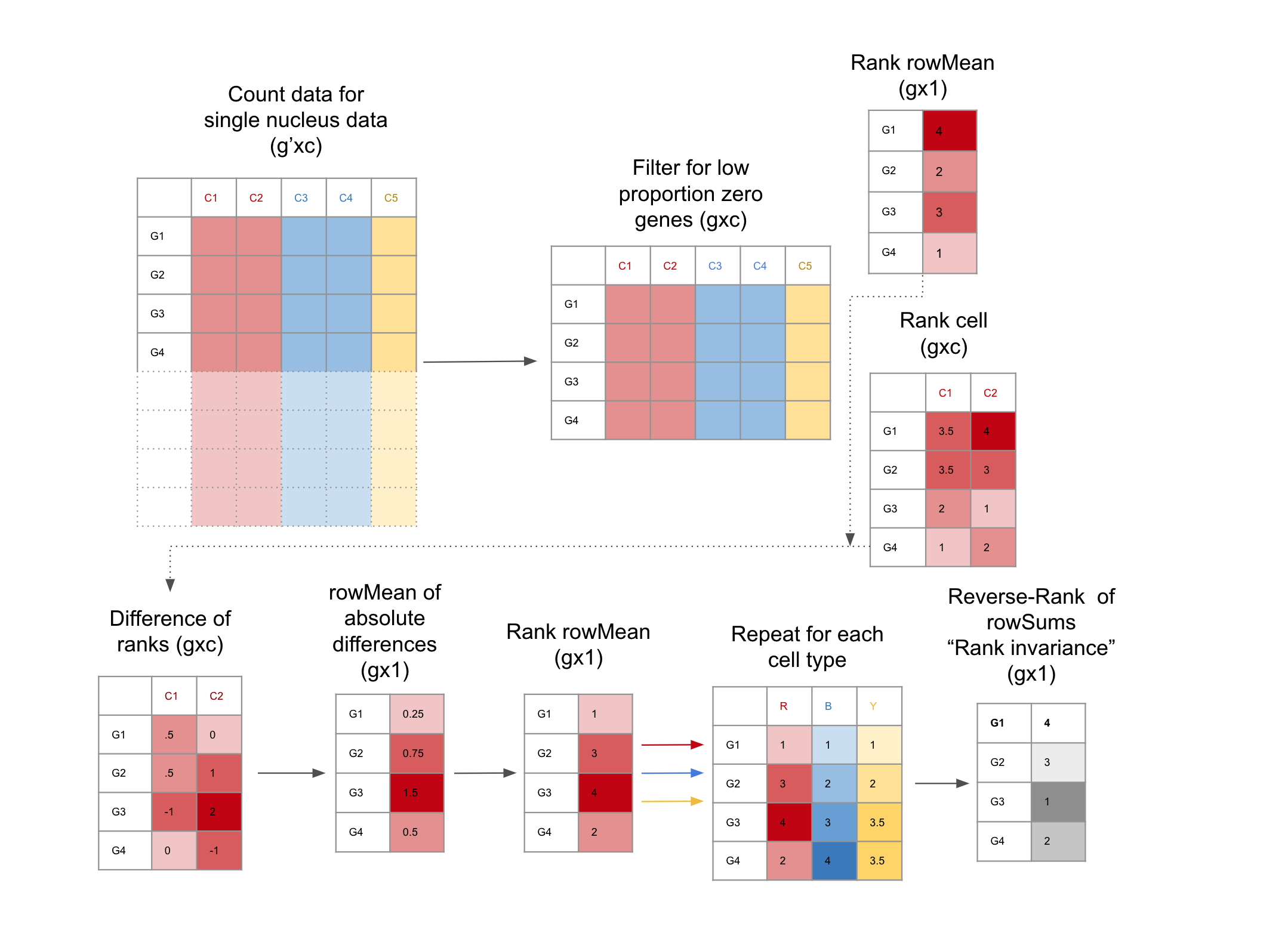
2. Evaluate genes for Rank Invariance The nuclei are grouped only by cell type. Within each cell type, the mean expression for each gene is ranked, the result is a vector (length is the number of genes), using the function rank_group(). Then the expression of each gene is ranked for each nucleus,the result is a matrix (the number of nuclei x number of genes), using the function rank_cells().Then the absolute difference between the rank of each nucleus and the mean expression is found, from here the mean of the differences for each gene is calculated, then ranked. These steps are repeated for each group, the result is a matrix of ranks, (number of cell types x number of genes). From here the sum of the ranks for each gene are reversed ranked, so there is one final value for each gene, the “Rank Invariance” The genes with the highest rank-invariance are considered good candidates as TREGs. This is calculated with rank_invariance_express(). This full process is implemented by: rank_invariance_express().

Example TREG Application

In this example we will apply our data driven process for TREG discovery to a snRNA-seq dataset. This process has three main steps:
1. Data prep
2. Gene filtering: dropping genes with low expression and high Proportion Zero (Equation \@ref(eq:propZero))
3. Rank Invariance Calculation

Load Packages

library("SingleCellExperiment")
library("pheatmap")
library("dplyr")
library("ggplot2")
library("tidyr")
library("tibble")

Download and Prep Data

Here we download a public single nucleus RNA-seq (snRNA-seq) data from r Citep(bib[['tran2021']]) that we'll use as our example. This data can be accessed on github. This data is from postmortem human brain in the dorsolateral prefrontal cortex (DLPFC) region, and contains gene expression data for 11k nuclei.

We will use BiocFileCache() to cache this data. It is stored as a SingleCellExperiment object named sce.dlpfc.tran, and takes 1.01 GB of RAM memory to load.

# Download and save a local cache of the data available at:
# https://github.com/LieberInstitute/10xPilot_snRNAseq-human#processed-data
bfc <- BiocFileCache::BiocFileCache()
url <- paste0(
    "https://libd-snrnaseq-pilot.s3.us-east-2.amazonaws.com/",
    "SCE_DLPFC-n3_tran-etal.rda"
)
local_data <- BiocFileCache::bfcrpath(url, x = bfc)

load(local_data, verbose = TRUE)

## Using 1.01 GB
# lobstr::obj_size(sce.dlpfc.tran)

ct_names <- tibble(
    "Cell Type" = c(
        "Astrocyte",
        "Excitatory Neurons",
        "Microglia",
        "Oligodendrocytes",
        "Oligodendrocyte Progenitor Cells",
        "Inhibitory Neurons"
    ),
    "Acronym" = c(
        "Astro",
        "Excit",
        "Micro",
        "Oligo",
        "OPC",
        "Inhib"
    )
)

knitr::kable(ct_names, caption = "Cell type names and corresponding acronyms used in this dataset", label = "acronyms")

Human brain tissue consists of many types of cells, for the porpose of this demo, we will focus on the six major cell types listed in Table \@ref(tab:acronyms).

Filter and Refine to Cell Types of Interest

First we will combine all of the Excit, Inhib subtypes, as it is a finer resolution than we want to examine, and combine rare subtypes in to one group. If there are too few cells in a group there may not be enough data to get good results. This new cell type classification is stored in the colData as cellType.broad.

## Explore the dimensions and cell type annotations
dim(sce.dlpfc.tran)
table(sce.dlpfc.tran$cellType)

## Use a lower resolution of cell type annotation
sce.dlpfc.tran$cellType.broad <- gsub("_[A-Z]$", "", sce.dlpfc.tran$cellType)
(cell_type_tab <- table(sce.dlpfc.tran$cellType.broad))

Next, we will drop any groups with < 50 cells after merging subtypes. This excludes any very rare cell types. Now we are working with the six broad cell types we are interested in.

## Find cell types with < 50 cells
(ct_drop <- names(cell_type_tab)[cell_type_tab < 50])

## Filter columns of sce object
sce.dlpfc.tran <- sce.dlpfc.tran[, !sce.dlpfc.tran$cellType.broad %in% ct_drop]

## Check new cell type bread down and dimension
table(sce.dlpfc.tran$cellType.broad)

dim(sce.dlpfc.tran)

Filter Genes

Single Nucleus data is often very sparse (lots of zeros in the count data), this dataset is 88% sparse. We can illustrate this in the heat map of the first 1k genes and 500 cells. The heatmap is mostly blue, indicating low values (Figure \@ref(fig:examineSparsity)).

## this data is 88% sparse
sum(assays(sce.dlpfc.tran)$counts == 0) / (nrow(sce.dlpfc.tran) * ncol(sce.dlpfc.tran))

## lets make a heatmap of the first 1k genes and 500 cells
count_test <- as.matrix(assays(sce.dlpfc.tran)$logcounts[seq_len(1000), seq_len(500)])
pheatmap(count_test,
    cluster_rows = FALSE,
    cluster_cols = FALSE,
    show_rownames = FALSE,
    show_colnames = FALSE
)

Filter to Top 50% Expression

Determine the median expression of genes over all rows, drop all the genes that are below this limit.

row_means <- rowMeans(assays(sce.dlpfc.tran)$logcounts)
(median_row_means <- median(row_means))

sce.dlpfc.tran <- sce.dlpfc.tran[row_means > median_row_means, ]
dim(sce.dlpfc.tran)

After this filter lets check sparsity and make a heatmap of the first 1k genes and 500 cells. We are seeing more non-blue (Figure \@ref(fig:top50FilterHeatmap))!

## this data down to 77% sparse
sum(assays(sce.dlpfc.tran)$counts == 0) / (nrow(sce.dlpfc.tran) * ncol(sce.dlpfc.tran))

## replot heatmap
count_test <- as.matrix(assays(sce.dlpfc.tran)$logcounts[seq_len(1000), seq_len(500)])
pheatmap::pheatmap(count_test,
    cluster_rows = FALSE,
    cluster_cols = FALSE,
    show_rownames = FALSE,
    show_colnames = FALSE
)

Calculate Proportion Zero and Pick Cutoff

For each group (let's use cellType.broad) get the Proportion Zero for each gene, where Proportion Zero is defined in Equation \@ref(eq:propZero) where $c_{i,j,k,z}$ is the number of snRNA-seq counts for cell/nucleus $z$ for gene $i$, cell type $j$, brain region $k$, and $n_{j, k}$ is the number of cells/nuclei for cell type $j$ and brain region $k$.

\begin{equation} PZ_{i,j,k} = \sum_{z=1}^{n_{j,k}} I(c_{i,j,k} > 0) / n_{j,k} (#eq:propZero) \end{equation}

# get prop zero for each gene for each cell type
prop_zeros <- get_prop_zero(sce.dlpfc.tran, group_col = "cellType.broad")
head(prop_zeros)

To determine a good cutoff for filtering lets examine the distribution of these Proportion Zeros by group.

# Pivot data longer for plotting
prop_zero_long <- prop_zeros %>%
    rownames_to_column("Gene") %>%
    pivot_longer(!Gene, names_to = "Group", values_to = "prop_zero")

# Plot histograms
(prop_zero_histogram <- ggplot(
    data = prop_zero_long,
    aes(x = prop_zero, fill = Group)
) +
    geom_histogram(binwidth = 0.05) +
    facet_wrap(~Group))

Looks like around 0.9 the densities peak, we'll set that as the cutoff (Figure \@ref(fig:propZeroDistribution)).

## Specify a cutoff, here we use 0.9
propZero_limit <- 0.9

## Add a vertical red dashed line where the cutoff is located
prop_zero_histogram +
    geom_vline(xintercept = propZero_limit, color = "red", linetype = "dashed")

The chosen cutoff excludes the peak Proportion Zeros from all groups (Figure \@ref(fig:pickCutoff)).

Filter by the Max Proportion Zero

Use the cutoff to filter the remaining genes. Only 4k or ~11% of genes pass with this cutoff. Filter the SCE object to this set of genes.

## get a list of filtered genes
filtered_genes <- filter_prop_zero(prop_zeros, cutoff = propZero_limit)

## How many genes pass the filter?
length(filtered_genes)

## What % of genes is this
length(filtered_genes) / nrow(sce.dlpfc.tran)

## Filter the sce object
sce.dlpfc.tran <- sce.dlpfc.tran[filtered_genes, ]

One last check of the sparsity, more non-blue means more non-zero values for the Rank Invariance calculation, which prevents rank ties (Figure \@ref(fig:propZeroFilterHeatmap)).

## this data down to 50% sparse
sum(assays(sce.dlpfc.tran)$counts == 0) / (nrow(sce.dlpfc.tran) * ncol(sce.dlpfc.tran))

## re-plot heatmap
count_test <- as.matrix(assays(sce.dlpfc.tran)$logcounts[seq_len(1000), seq_len(500)])
pheatmap::pheatmap(count_test,
    cluster_rows = FALSE,
    cluster_cols = FALSE,
    show_rownames = FALSE,
    show_colnames = FALSE
)

Run Rank Invariance

To get the Rank Invariance (RI), the rank of the genes across the cells in a group, and between groups is considered. One way to calculate RI is to find the group rank values, and cell rank values separately, then combine them as shown below. The genes with the top RI values are the best candidate TREGs.

## Get the rank of the gene in each group
group_rank <- rank_group(sce.dlpfc.tran, group_col = "cellType.broad")

## Get the rank of the gene for each cell
cell_rank <- rank_cells(sce.dlpfc.tran, group_col = "cellType.broad")

## Use both rankings to calculate rank_invariance()
rank_invar <- rank_invariance(group_rank, cell_rank)

## The top 5 Candidate TREGs:
head(sort(rank_invar, decreasing = TRUE))

The rank_invariance_express() function combines these three steps into one function, and achieves the same results.

## rank_invariance_express() runs the previous functions for you
rank_invar2 <- rank_invariance_express(
    sce.dlpfc.tran,
    group_col = "cellType.broad"
)
## Again the top 5 Candidate TREGs:
head(sort(rank_invar2, decreasing = TRUE))

## Check computationally that the results are identical
stopifnot(identical(rank_invar, rank_invar2))

The rank_invariance_express() function is more efficient as well, as it loops through the data to rank the genes over cells, and groups at the same time.

Selecting thresholds

When identifying candidate TREGs with our software, there are a few thresholds users will select. In our manuscript r Citep(bib[['TREGpaper']]), we used a few filters.

1. We focused on genes among the top 50% of genes expressed in the snRNA-seq data. This helped address sparsity inherent to snRNA-seq data.
2. We used a maximum Proportion Zero filter of 75%.

Overall it’s a balancing act between the computational requirements (reduce sparsity inherent to snRNA-seq data, reduce expression rank ties) and the biological goal (select a gene expressed in most nuclei from all cell types of interest). If you focus on just genes expressed in all nuclei or above a given threshold as shown in this figure, you could be losing too many genes (likely no gene is expressed in all nuclei as shown in our data) or genes that are not expressed at all in some cell types, given that some cell types are much less frequent than other cell types. While we consider the thresholds we used as those that balance both aspects and are practical, ultimately we do encourage users to plot their own data.

For example, making plots like those from Supplementary Figure 2. Supplementary Figure 2A is useful to examine whether genes you might have expected to pass the filters are being dropped. You can then check they were just below the filtering cutoffs, or significantly far away from them. Once you have the candidate TREG results, then Supplementary Figure 2B is useful to examine at what point do the top candidate TREGs have a stronger relationship with total RNA expression as measured from the snRNA-seq data. That is, where the blue curve jumps up and shows a more clear association between the two axes of that plot.

Among the top candidate TREGs, there might be practical limitations to consider for using that TREG in another assay, such as availability of RNAscope probes as well as measurability of the puncta for a given probe. We showed in Figure 5 how MALAT1 could not be reliably quantified with RNAscope due to high expression and oversaturation of fluorescent signals. In the case of RNAscope, we recommend testing the measurability of candidate TREGs with RNAscope data before generating a full dataset with a probe that may be difficult to accurately quantify.

Conclusion

We have identified top candidate TREG genes from this dataset, by applying Proportion Zero filtering and calculating the Rank Invariance using the TREG package. This provides a list of candidate genes that can be useful for estimating total RNA expression in assays such as smFISH.

However, we are unable to assess other important qualities of these genes that ensure they are experimentally compatible with the chosen assay. For example, in smFISH with RNAscope it is important that a TREG be expressed at a level that individual puncta can be accurately counted, and have a dynamic range of puncta. During experimental validation we found that MALAT1 was too highly expressed in the human DLPFC to segment individual puncta, and ruled it out as an experimentally useful TREG r Citep(bib[['TREGpaper']]).

Therefore, we recommend that TREGs be evaluated in the assay or analysis of choice you perform a validation experiment with a pilot sample before implementing experiments using it on rare and valuable samples.

If you are designing a sc/snRNA-seq study to use as a reference for deconvolution of bulk RNA-seq, we recommend that you generate spatially-adjacent dissections in order to use them for RNAscope experiments. By doing so, you could identify cell types in your sc/snRNA-seq data, then identify candidate TREGs based on those cell types, and use these candidate TREGs in your spatially-adjacent dissections to quantify size and total RNA amounts for the cell types of interest r Citep(bib[['TREGpaper']]). Furthermore, the RNAscope data alone can be used as a gold standard reference for cell fractions.

TREGs could be useful for other research purposes and other contexts than the ones we envisioned!

Thanks for your interest in TREGs :)

Reproducibility

The r Biocpkg('TREG') package r Citep(bib[['TREG']]) was made possible thanks to:

• R r Citep(bib[['R']])
• r Biocpkg('BiocFileCache') r Citep(bib[['BiocFileCache']])
• r Biocpkg('BiocStyle') r Citep(bib[['BiocStyle']])
• r CRANpkg('dplyr') r Citep(bib[['dplyr']])
• r CRANpkg('ggplot2') r Citep(bib[['ggplot2']])
• r CRANpkg('knitr') r Citep(bib[['knitr']])
• r CRANpkg('Matrix') r Citep(bib[['Matrix']])
• r CRANpkg('pheatmap') r Citep(bib[['pheatmap']])
• r CRANpkg('purrr') r Citep(bib[['purrr']])
• r CRANpkg('rafalib') r Citep(bib[['rafalib']])
• r CRANpkg("RefManageR") r Citep(bib[["RefManageR"]])
• r CRANpkg('rmarkdown') r Citep(bib[['rmarkdown']])
• r CRANpkg('sessioninfo') r Citep(bib[['sessioninfo']])
• r Biocpkg('SummarizedExperiment') r Citep(bib[['SummarizedExperiment']])
• r CRANpkg('testthat') r Citep(bib[['testthat']])
• r CRANpkg('tibble') r Citep(bib[['tibble']])
• r CRANpkg('tidyr') r Citep(bib[['tidyr']])

Code for creating the vignette

## Create the vignette
library("rmarkdown")
system.time(render("finding_Total_RNA_Expression_Genes.Rmd"))

## Extract the R code
library("knitr")
knit("finding_Total_RNA_Expression_Genes.Rmd", tangle = TRUE)

Date the vignette was generated.

## Date the vignette was generated
Sys.time()

Wallclock time spent generating the vignette.

## Processing time in seconds
totalTime <- diff(c(startTime, Sys.time()))
round(totalTime, digits = 3)

R session information.

## Session info
library("sessioninfo")
options(width = 120)
session_info()

Bibliography

This vignette was generated using r Biocpkg('BiocStyle') r Citep(bib[['BiocStyle']]), r CRANpkg('knitr') r Citep(bib[['knitr']]) and r CRANpkg('rmarkdown') r Citep(bib[['rmarkdown']]) running behind the scenes.

Citations made with r CRANpkg('RefManageR') r Citep(bib[['RefManageR']]).

## Print bibliography
PrintBibliography(bib, .opts = list(hyperlink = "to.doc", style = "html"))

LieberInstitute/TREG documentation built on May 7, 2024, 3:49 p.m.