README.md

In McCartneyAC/mccrr: Personal R Package

mccrr

A Personal R package

This package contains objects and functions that I have found via the #rstats community and some things I have developed myself. These are functions and objects I use on a regular basis and so have committed to a package for ease of access. Where possible, credit is given to the original poster.

Name

The name derives from Yihui Xie's joke about how Hadley Wickham derives his r package names:

tidy_name = function(x) {
  x = tolower(substr(abbreviate(x), 1, 4))
  paste(c(x, rep('r', 5 - nchar(x))), collapse = '')
}

Data

This package contains the "teacher_pay" data set which contains by-state data on teacher pay (real and COLA) as well as some political and demographic information about the state. Can be used as a toy data set or joined with other data for more structured analyses by state.

Some Notable Functions:

Here are some that I tend to use more frequently or advertise to friends when they need them.

Center

Centers a variable on a given center. Should be useable within a tidy data pipe, e.g.

hsb %>%
  center(ses, mean(ses))
# or 
hsb %>%
  center(mathach, 5)

The first example above does a grand-mean center; however, often in HLM we need to group mean center. This is easily accomplished:

hsb %>% 
  group_by(schoolid) %>% 
  center(mathach, mean(mathach)) 

Correlate

A tidy / pipeable alias of base::cor(), with the added default to delete pairwise-incomplete-observations. Allows additional arguments to be passed to base::cor() to allow for, e.g. Spearman rather than Pearson.

> teacher_pay %>% 
+   correlate(clinton_votes_2016, adjusted_pay)
                   adjusted_pay
clinton_votes_2016    0.3040241

Dossier

Generates a dossier for a given observation in your data set. For example, if you have an id variable and an observation with an id number of "1234", then:

df %>%
  dossier(id = "1234")

Or using the data from my Teacher_pay package:

dat_full %>% 
   mccrr::dossier(abbreviation, "SC")
                   [,1]            
state              "South Carolina"
abbreviation       "SC"            
adjusted_pay       "52878"         
actual_pay         "48542"         
strike2018_2019    "1"             
clinton_votes_2016 "849469"        
trump_votes_2016   "1143611"       
population2018     "5084127"       
percent_union2018  "3.6"           
pct_clinton        "16.70826"      
pct_trump          "22.49375"      
log_pop            "6.706216"      
division           "5"             
div_name           "South_Atlantic"
pct_white_2012     "63.9"          
adj                "91.79999"      
margin             "-5.785497"   

Paste Data

It's probably a terrible idea to do this on a regular basis or with any important data analysis you'll ever need again, but if you want to quickly copy and paste a data set from excel into R, you can use this without any arguments, as follows:

dat <- paste_data()

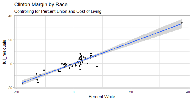
Added Variable Plot

This should have been standardized in R long ago and arguably ought to have been an initial geom_ in ggplot2, but here we are: Define your full model and your restricted model, then build any other ggplot formatting you want around your model later, as such:

mod6 <- dat_full %>% 
  lmer(margin ~ 1 + percent_union2018*adj + log_pop + pct_white_2012 +(1|div_name), data = .)
mod6_restricted <- dat_full %>% 
  lmer(margin ~ 1 + percent_union2018*adj + log_pop  +(1|div_name), data = .)

gg_added_var(partial= mod6_restricted, extended = mod6) + 
  labs(title = "Clinton Margin by Race", 
       subtitle = "Controlling for Percent Union and Cost of Living",
       x = "Percent White") + 
  theme_light()

"Not in"

Just the logical opposite of the %in% infix operator, which is sometimes useful. For example, if you have a list of hero characters separate from your character dataset and you want to find only the non-hero characters:

villains <- characters %>%
  filter(name %notin% heros_list)

Statar

The package currently contains some functions that are intended to bridge the code-switching problem when working in both Stata and R. stata_summary gives regression output in stata's format. Additional functions exist for common data manipulations that have different names in the two languages, e.g. stata_regress for lm() and stata_browse for View() (Also view() for View() in this package. Sometimes you just get confused and type the wrong thing. The package is here to help. stata_use() is particularly helpful because it will parse your data file for filetype and return a tibble, making it a generic read_ function.

to add:

https://multithreaded.stitchfix.com/blog/2017/06/15/beware-r-in-production/

A "control F" Function that uses filter with contains (text) to find all rows containing a certain string.

Add this on next update:

decumulate<-function(df, var){
  user_var<-enquo(var)
  varname <- quo_name(user_var)
  firstval<-df %>% 
    # how does get_quo_expr help here?
    dplyr::select(!!user_var) %>% 
    dplyr::filter(row_number()==1)

  mutate(df, `:=`(!!varname, (
    # actual function here
    c(firstval, diff(!!user_var))
  ))) %>% 
    unnest(!!user_var)
}

• this function is not currently working as intended in all scenarios. Needs further testing and debugging.

put this in next iteration:

# degrees to radians
deg2rad<-function(d){
  return(d * (pi/180))
}

# calculate haversine distance between two coordinates. 
haversine_km<-function(lat1,lon1,lat2,lon2){
  Rad <- 6371 # Radius of earth in km
  dLat <- deg2rad(lat2-lat1)
  dLon <- deg2rad(lon2-lon1)
  a <- sin(dLat/2)*sin(dLat/2) + cos(deg2rad(lat1)) * cos(deg2rad(lat2)) * sin(dLon/2) * sin(dLon/2)
  c <- 2 * atan2(sqrt(a), sqrt(1-a))
  d <- Rad*c # distance in km
  return(d)
}

Shocked at how often haversine distance comes up.

McCartneyAC/mccrr documentation built on March 24, 2024, 5:12 p.m.