inst/examples/appendices/simulation_example.md

In cboettig/earlywarning: Detection of Early Warning Signals for Catastrophic Bifurcations

render_gfm()  # use GFM hooks for output
opts_knit$set(base.url = "https://github.com/cboettig/earlywarning/wiki/")

Clear our working space and load the earlywarning package.

require(earlywarning)

## Loading required package: earlywarning

We load the data set

data(ibms)
A <- stability_model(ibm_critical, "OU")
B <- stability_model(ibm_critical, "LSN")
observed <- -2 * (logLik(A) - logLik(B))

Now we set up the parallel environment...

require(snowfall)

## Loading required package: snowfall

## Loading required package: snow

sfInit(par = T, cpu = 16)

## R Version:  R version 2.14.1 (2011-12-22) 
## 

## snowfall 1.84 initialized (using snow 0.3-8): parallel execution on 16 CPUs.
## 

sfLibrary(earlywarning)

## Library earlywarning loaded.

## Library earlywarning loaded in cluster.
## 

sfExportAll()

reps <- sfLapply(1:100, function(i) compare(A, 
    B))

... because the next step can take a while. compare simulates under each model, and then estimates both models on both simulated sets of data (for a total of 4 model fits). As only the LSN fit is computationally intensive, this takes about twice the time as the above fitting step of model B. We will then repeat this many times to build up a bootstrap distribution.

We illustrate this step with the parallel loop function parLapply from the snow package, a mature parallelization toolbox ( e.g. see Schmidberger et al., 2009) which works well in parallel on a multicore chip, or in parallel across a large cluster (via MPI). Rather than build this choice into the earlywarning signals package, the user can choose whatever looping implementation they desire to compute replicates of the comparison. Though this example was run on a cluster of 100 nodes, though users willing to wait a few days could easily run this on a typical laptop. Our results are cached in the package, so anyone seeking to explore this example can run data(example_analysis) instead.

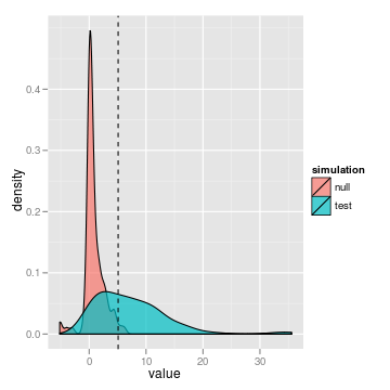
Once this step is finished, the remaining analysis is just a matter of shuffling and plotting the data. We extract the likelihood ratios (deviances) from the null and test simulations with a simple function.

lr <- lik_ratios(reps)

We can visualize this data as overlapping distributions

require(ggplot2)

## Loading required package: ggplot2

## Loading required package: reshape

## Loading required package: plyr

## 
## Attaching package: 'reshape'
## 

## The following object(s) are masked from 'package:plyr':
## 
##     rename, round_any
## 

## Loading required package: grid

## Loading required package: proto

ggplot(lr) + geom_density(aes(value, fill = simulation), 
    alpha = 0.7) + geom_vline(xintercept = observed, lty = 2)

Or as beanplot

require(beanplot)

## Loading required package: beanplot

beanplot(value ~ simulation, lr, what = c(0, 1, 
    0, 0))

## Error: could not find function "beanplot"

abline(h = observed, lty = 2)

## Error: plot.new has not been called yet

We can make the ROC curve by calculating the true and false positive rates from the overlap of these distributions using roc_data. This gives us a data frame of threshold values for our statistic, and the corresponding false positive rate and true positive rate. We can simply plot those rates against each other to create the ROC curve.

roc <- roc_data(lr)

## Area Under Curve =  0.865705222090351

## True positive rate =  0.58 at false positive rate of 0.02

ggplot(roc) + geom_line(aes(False.positives, True.positives), 
    lwd = 1)

## Error: object 'False.positives' not found

We can also look at the bootstraps of the parameters. Another helper function will reformat this data from reps list. The fit column uses a two-letter code to indicate first what model was used to simulate the data, and then what model was fit to the data. For instance, AB means the data was simulated from model A (the null, OU model) but fit to B.

pars <- parameter_bootstraps(reps)
head(pars)

##     value parameter fit rep
## 1   1.380        Ro  AA   1
## 2 583.109     theta  AA   1
## 3 147.015     sigma  AA   1
## 4   1.631        Ro  AB   1
## 5 602.484     theta  AB   1
## 6 130.060     sigma  AB   1

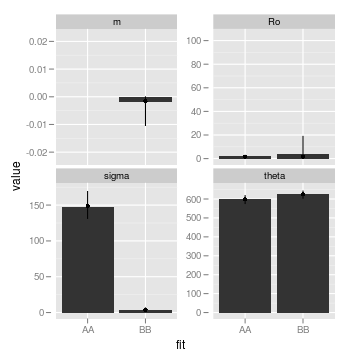
There are lots of options for visualizing this relatively high-dimensional data, which we can easily explore with a few commands from the ggplot2 package. For instance, we can look at average and range of parameters estimated in the bootstraps of each model:

require(Hmisc)

## Loading required package: Hmisc

## Loading required package: survival

## Loading required package: splines

## Hmisc library by Frank E Harrell Jr
## 
## Type library(help='Hmisc'), ?Overview, or ?Hmisc.Overview')
## to see overall documentation.
## 
## NOTE:Hmisc no longer redefines [.factor to drop unused levels when
## subsetting.  To get the old behavior of Hmisc type dropUnusedLevels().
## 

## 
## Attaching package: 'Hmisc'
## 

## The following object(s) are masked from 'package:survival':
## 
##     untangle.specials
## 

## The following object(s) are masked from 'package:plyr':
## 
##     is.discrete, summarize
## 

## The following object(s) are masked from 'package:base':
## 
##     format.pval, round.POSIXt, trunc.POSIXt, units
## 

ggplot(subset(pars, fit %in% c("AA", "BB")), aes(fit, 
    value)) + stat_summary(fun.y = mean, geom = "bar", position = "dodge") + 
    stat_summary(fun.data = median_hilow, geom = "pointrange", 
        position = position_dodge(width = 0.9), conf.int = 0.95) + 
    facet_wrap(~parameter, scales = "free_y")

We can easily repeat this code for the other data sets used in the study, which takes about six lines of code. While one could always use fewer lines, this keeps the steps explicit: (1) fit the null model, (2) fit the test model (3) check the observed likelihood ratio, (4) bootstrap, (5) get likelihood ratio distributions from the bootstraps, (6) convert the distribution into error rates.

data("chemostat")
A.chemo <- stability.model(chemostat, "OU")
B.chemo <- stability.model(chemostat, "LSN")
observed.chemo <- -2 * (logLik(A.chemo) - logLik(B.chemo))
reps.chemo <- sfLapply(1:100, function(i) compare(A.chemo, 
    B.chemo))
lr.chemo <- lik_ratios(reps.chemo)
roc.chemo <- roc_data(lr.chemo)

cboettig/earlywarning documentation built on May 13, 2019, 2:07 p.m.