inst/examples/BUGS/parametric-vs-nonparametric.md
In cboettig/nonparametric-bayes: Nonparametric Bayes inference for ecological models
Comparison of Nonparametric Bayesian Gaussian Process estimates to standard the Parametric Bayesian approach
Plotting and knitr options, (can generally be ignored)
require(modeest)
posterior.mode <- function(x) {
  mlv(x, method="shorth")$M
}
Model and parameters
f <- Myers
p <- c(1, 2, 6)
K <- 5  # approx, a li'l' less
allee <- 1.2 # approx, a li'l' less
Various parameters defining noise dynamics, grid, and policy costs.
sigma_g <- 0.05
sigma_m <- 0.0
z_g <- function() rlnorm(1, 0, sigma_g)
z_m <- function() 1+(2*runif(1, 0,  1)-1) * sigma_m
x_grid <- seq(0, 1.5 * K, length=50)
h_grid <- x_grid
profit <- function(x,h) pmin(x, h)
delta <- 0.01
OptTime <- 50  # stationarity with unstable models is tricky thing
reward <- 0
xT <- 0
Xo <-  allee+.5# observations start from
x0 <- K # simulation under policy starts from
Tobs <- 40
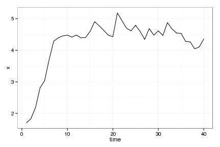
Sample Data
  set.seed(1234)
  #harvest <- sort(rep(seq(0, .5, length=7), 5))
  x <- numeric(Tobs)
  x[1] <- Xo
  nz <- 1
  for(t in 1:(Tobs-1))
    x[t+1] = z_g() * f(x[t], h=0, p=p)
  obs <- data.frame(x = c(rep(0,nz),
                          pmax(rep(0,Tobs-1), x[1:(Tobs-1)])),
                    y = c(rep(0,nz),
                          x[2:Tobs]))
raw_plot <- ggplot(data.frame(time = 1:Tobs, x=x), aes(time,x)) + geom_line()
raw_plot
Maximum Likelihood
set.seed(12345)
estf <- function(p){
    mu <- f(obs$x,0,p)
    -sum(dlnorm(obs$y, log(mu), p[4]), log=TRUE)
}
par <- c(p[1]*rlnorm(1,0,.2),
         p[2]*rlnorm(1,0,.1),
         p[3]*rlnorm(1,0, .1),
         sigma_g * rlnorm(1,0,.3))
o <- optim(par, estf, method="L", lower=c(1e-5,1e-5,1e-5,1e-5))
f_alt <- f
p_alt <- c(as.numeric(o$par[1]), as.numeric(o$par[2]), as.numeric(o$par[3]))
sigma_g_alt <- as.numeric(o$par[4])

est <- list(f = f_alt, p = p_alt, sigma_g = sigma_g_alt, mloglik=o$value)
Mean predictions
true_means <- sapply(x_grid, f, 0, p)
est_means <- sapply(x_grid, est$f, 0, est$p)
Non-parametric Bayes
#inv gamma has mean b / (a - 1) (assuming a>1) and variance b ^ 2 / ((a - 2) * (a - 1) ^ 2) (assuming a>2)
s2.p <- c(5,5)
d.p = c(10, 1/0.1)
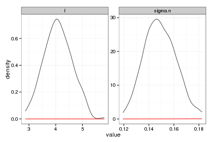
Estimate the Gaussian Process (nonparametric Bayesian fit)
gp <- gp_mcmc(obs$x, y=obs$y, n=1e5, s2.p = s2.p, d.p = d.p)
gp_dat <- gp_predict(gp, x_grid, burnin=1e4, thin=300)
Show traces and posteriors against priors
plots <- summary_gp_mcmc(gp, burnin=1e4, thin=300)

# Summarize the GP model
tgp_dat <-
    data.frame(  x = x_grid,
                 y = gp_dat$E_Ef,
                 ymin = gp_dat$E_Ef - 2 * sqrt(gp_dat$E_Vf),
                 ymax = gp_dat$E_Ef + 2 * sqrt(gp_dat$E_Vf) )
Parametric Bayesian Models
We use the JAGS Gibbs sampler, a recent open source BUGS
implementation with an R interface that works on most platforms.
We initialize the usual MCMC parameters; see ?jags for details.
All parametric Bayesian estimates use the following basic parameters for the JAGS MCMC:
y <- x
N <- length(x);
jags.data <- list("N","y")
n.chains <- 6
n.iter <- 1e6
n.burnin <- floor(10000)
n.thin <- max(1, floor(n.chains * (n.iter - n.burnin)/1000))
n.update <- 10
We will use the same priors for process and observation noise in each model,
stdQ_prior_p <- c(1e-6, 100)
stdR_prior_p <- c(1e-6, .1)
stdQ_prior  <- function(x) dunif(x, stdQ_prior_p[1], stdQ_prior_p[2])
stdR_prior  <- function(x) dunif(x, stdR_prior_p[1], stdR_prior_p[2])
Parametric Bayes of correct (Allen) model
We initiate the MCMC chain (init_p) using the true values of the
parameters p from the simulation. While impossible in real data, this
gives the parametric Bayesian approach the best chance at succeeding.
y is the timeseries (recall obs has the $x_t$, $x_{t+1}$ pairs)
The actual model is defined in a model.file that contains an R function
that is automatically translated into BUGS code by R2WinBUGS. The file
defines the priors and the model. We write the file from R as follows:
K_prior_p <- c(0.01, 20.0)
r0_prior_p <- c(0.01, 6.0)
theta_prior_p <- c(0.01, 20.0)

bugs.model <-
paste(sprintf(
"model{
  K     ~ dunif(%s, %s)
  r0    ~ dunif(%s, %s)
  theta ~ dunif(%s, %s)
  stdQ ~ dunif(%s, %s)",
  K_prior_p[1], K_prior_p[2],
  r0_prior_p[1], r0_prior_p[2],
  theta_prior_p[1], theta_prior_p[2],
  stdQ_prior_p[1], stdQ_prior_p[2]),

  "
  iQ <- 1 / (stdQ * stdQ);
  y[1] ~ dunif(0, 10)
  for(t in 1:(N-1)){
    mu[t] <- log(y[t]) + r0 * (1 - y[t]/K)* (y[t] - theta) / K
    y[t+1] ~ dlnorm(mu[t], iQ)
  }
}")
writeLines(bugs.model, "allen_process.bugs")
Write the priors into a list for later reference
K_prior     <- function(x) dunif(x, K_prior_p[1], K_prior_p[2])
r0_prior <- function(x) dunif(x, r0_prior_p[1], r0_prior_p[2])
theta_prior <- function(x) dunif(x, theta_prior_p[1], theta_prior_p[2])
par_priors  <- list(K = K_prior, deviance = function(x) 0 * x,
                    r0 = r0_prior, theta = theta_prior,
                    stdQ = stdQ_prior)
We define which parameters to keep track of, and set the initial values of
parameters in the transformed space used by the MCMC. We use logarithms
to maintain strictly positive values of parameters where appropriate.
jags.params=c("K","r0","theta","stdQ") # be sensible about the order here
jags.inits <- function(){
  list("K"= 8 * rlnorm(1,0, 0.1),
       "r0"= 2 * rlnorm(1,0, 0.1) ,
       "theta"=   5 * rlnorm(1,0, 0.1) ,
       "stdQ"= abs( 0.1 * rlnorm(1,0, 0.1)),
       .RNG.name="base::Wichmann-Hill", .RNG.seed=123)
}

set.seed(1234)
# parallel refuses to take variables as arguments (e.g. n.iter = 1e5 works, but n.iter = n doesn't)
allen_jags <- do.call(jags.parallel, list(data=jags.data, inits=jags.inits,
                                      jags.params, n.chains=n.chains,
                                      n.iter=n.iter, n.thin=n.thin,
                                      n.burnin=n.burnin,
                                      model.file="allen_process.bugs"))

# Run again iteratively if we haven't met the Gelman-Rubin convergence criterion
recompile(allen_jags) # required for parallel
allen_jags <- do.call(autojags,
                                            list(object=allen_jags, n.update=n.update,
                           n.iter=n.iter, n.thin = n.thin))
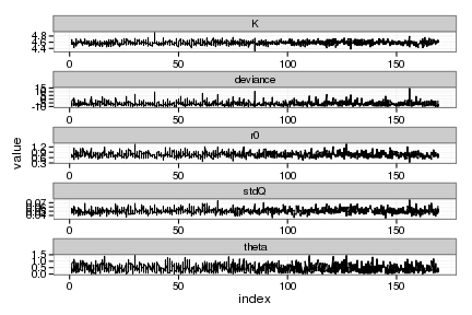
Convergence diagnostics for Allen model
R notes: this strips classes from the mcmc.list object (so that we have list of matrices; objects that reshape2::melt can handle intelligently), and then combines chains into one array. In this array each parameter is given its value at each sample from the posterior (index) for each chain.
tmp <- lapply(as.mcmc(allen_jags), as.matrix) # strip classes the hard way...
allen_posteriors <- melt(tmp, id = colnames(tmp[[1]]))
names(allen_posteriors) = c("index", "variable", "value", "chain")
ggplot(allen_posteriors) + geom_line(aes(index, value)) +
  facet_wrap(~ variable, scale="free", ncol=1)
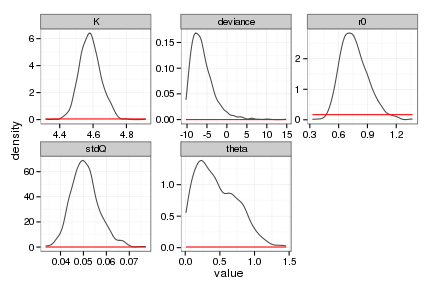
allen_priors <- ddply(allen_posteriors, "variable", function(dd){
    grid <- seq(min(dd$value), max(dd$value), length = 100)
    data.frame(value = grid, density = par_priors[[dd$variable[1]]](grid))
})

ggplot(allen_posteriors, aes(value)) +
  stat_density(geom="path", position="identity", alpha=0.7) +
  geom_line(data=allen_priors, aes(x=value, y=density), col="red") +
  facet_wrap(~ variable, scale="free", ncol=3)
Reshape the posterior parameter distribution data, transform back into original space, and calculate the mean parameters and mean function
A <- allen_posteriors
A$index <- A$index + A$chain * max(A$index) # Combine samples across chains by renumbering index
pardist <- acast(A, index ~ variable)
bayes_coef <- apply(pardist,2, posterior.mode)
bayes_pars <- unname(c(bayes_coef["r0"], bayes_coef["K"], bayes_coef["theta"])) # parameters formatted for f
allen_f <- function(x,h,p) unname(RickerAllee(x,h, unname(p[c("r0", "K", "theta")])))
allen_means <- sapply(x_grid, f, 0, bayes_pars)
bayes_pars
[1] 0.7082 4.5647 0.2558
head(pardist)
        K deviance     r0    stdQ  theta
170 4.531   -8.534 0.6867 0.04473 0.3832
171 4.516    1.335 0.6471 0.05928 1.0216
172 4.574   -8.576 0.8532 0.04983 0.7196
173 4.614   -6.873 0.5302 0.04611 0.1390
174 4.628   -5.580 0.7331 0.04024 0.5064
175 4.503   -7.443 0.7341 0.04474 0.2369
Parametric Bayes based on the structurally wrong model (Ricker)
K_prior_p <- c(0.01, 40.0)
r0_prior_p <- c(0.01, 20.0)
bugs.model <-
paste(sprintf(
"model{
  K    ~ dunif(%s, %s)
  r0    ~ dunif(%s, %s)
  stdQ ~ dunif(%s, %s)",
  K_prior_p[1], K_prior_p[2],
  r0_prior_p[1], r0_prior_p[2],
  stdQ_prior_p[1], stdQ_prior_p[2]),
  "
  iQ <- 1 / (stdQ * stdQ);
  y[1] ~ dunif(0, 10)
  for(t in 1:(N-1)){
    mu[t] <- log(y[t]) + r0 * (1 - y[t]/K)
    y[t+1] ~ dlnorm(mu[t], iQ)
  }
}")
writeLines(bugs.model, "ricker_process.bugs")
Compute prior curves
K_prior     <- function(x) dunif(x, K_prior_p[1], K_prior_p[2])
r0_prior <- function(x) dunif(x, r0_prior_p[1], r0_prior_p[2])
par_priors <- list(K = K_prior, deviance = function(x) 0 * x,
                   r0 = r0_prior, stdQ = stdQ_prior)
We define which parameters to keep track of, and set the initial values of
parameters in the transformed space used by the MCMC.
jags.params=c("K","r0", "stdQ")
jags.inits <- function(){
  list("K"=10 * rlnorm(1,0,.5),
       "r0"= rlnorm(1,0,.5),
       "stdQ"=sqrt(0.05) * rlnorm(1,0,.5),
       .RNG.name="base::Wichmann-Hill", .RNG.seed=123)
}
set.seed(12345)
ricker_jags <- do.call(jags.parallel,
                       list(data=jags.data, inits=jags.inits,
                            jags.params, n.chains=n.chains,
                            n.iter=n.iter, n.thin=n.thin, n.burnin=n.burnin,
                            model.file="ricker_process.bugs"))
recompile(ricker_jags)
Compiling model graph
   Resolving undeclared variables
   Allocating nodes
   Graph Size: 249

Initializing model

Compiling model graph
   Resolving undeclared variables
   Allocating nodes
   Graph Size: 249

Initializing model

Compiling model graph
   Resolving undeclared variables
   Allocating nodes
   Graph Size: 249

Initializing model

Compiling model graph
   Resolving undeclared variables
   Allocating nodes
   Graph Size: 249

Initializing model

Compiling model graph
   Resolving undeclared variables
   Allocating nodes
   Graph Size: 249

Initializing model

Compiling model graph
   Resolving undeclared variables
   Allocating nodes
   Graph Size: 249

Initializing model
ricker_jags <- do.call(autojags,
                       list(object=ricker_jags, n.update=n.update,
                                                        n.iter=n.iter, n.thin = n.thin,
                                                        progress.bar="none"))
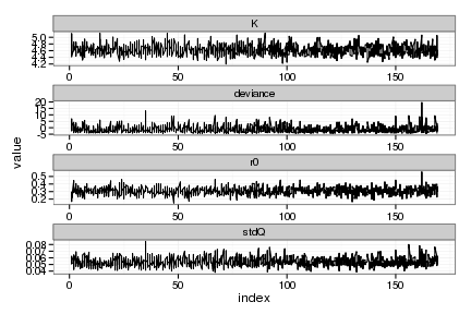
Convergence diagnostics for parametric bayes Ricker model
tmp <- lapply(as.mcmc(ricker_jags), as.matrix) # strip classes the hard way...
ricker_posteriors <- melt(tmp, id = colnames(tmp[[1]]))
names(ricker_posteriors) = c("index", "variable", "value", "chain")

ggplot(ricker_posteriors) + geom_line(aes(index, value)) +
  facet_wrap(~ variable, scale="free", ncol=1)
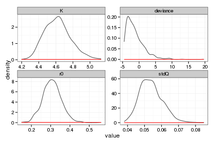
ricker_priors <- ddply(ricker_posteriors, "variable", function(dd){
    grid <- seq(min(dd$value), max(dd$value), length = 100)
    data.frame(value = grid, density = par_priors[[dd$variable[1]]](grid))
})
# plot posterior distributions
ggplot(ricker_posteriors, aes(value)) +
  stat_density(geom="path", position="identity", alpha=0.7) +
  geom_line(data=ricker_priors, aes(x=value, y=density), col="red") +
  facet_wrap(~ variable, scale="free", ncol=2)
Reshape posteriors data, transform back, calculate mode and corresponding function.
A <- ricker_posteriors
A$index <- A$index + A$chain * max(A$index) # Combine samples across chains by renumbering index
ricker_pardist <- acast(A, index ~ variable)
bayes_coef <- apply(ricker_pardist,2, posterior.mode)
ricker_bayes_pars <- unname(c(bayes_coef["r0"], bayes_coef["K"]))
ricker_f <- function(x,h,p){
  sapply(x, function(x){
    x <- pmax(0, x-h)
    pmax(0, x * exp(p["r0"] * (1 - x / p["K"] )) )
  })
}
ricker_means <- sapply(x_grid, Ricker, 0, ricker_bayes_pars[c(1,2)])
head(ricker_pardist)
        K deviance     r0    stdQ
170 4.796  -2.4558 0.2928 0.05125
171 4.604   4.2228 0.4464 0.06022
172 4.579  -3.6943 0.2798 0.05368
173 4.727   0.8348 0.2275 0.06162
174 4.686   0.1420 0.2346 0.04685
175 4.361  -0.5967 0.2783 0.05220
ricker_bayes_pars
[1] 0.302 4.597
Myers Parametric Bayes
r0_prior_p <- c(.0001, 10.0)
theta_prior_p <- c(.0001, 10.0)
K_prior_p <- c(.0001, 40.0)
bugs.model <-
paste(sprintf(
"model{
  r0    ~ dunif(%s, %s)
  theta    ~ dunif(%s, %s)
  K    ~ dunif(%s, %s)
  stdQ ~ dunif(%s, %s)",
  r0_prior_p[1], r0_prior_p[2],
  theta_prior_p[1], theta_prior_p[2],
  K_prior_p[1], K_prior_p[2],
  stdQ_prior_p[1], stdQ_prior_p[2]),

  "
  iQ <- 1 / (stdQ * stdQ);

  y[1] ~ dunif(0, 10)
  for(t in 1:(N-1)){
    mu[t] <- log(r0)  + theta * log(y[t]) - log(1 + pow(abs(y[t]), theta) / K)
    y[t+1] ~ dlnorm(mu[t], iQ)
  }
}")
writeLines(bugs.model, "myers_process.bugs")
K_prior     <- function(x) dunif(x, K_prior_p[1], K_prior_p[2])
r_prior     <- function(x) dunif(x, r0_prior_p[1], r0_prior_p[2])
theta_prior <- function(x) dunif(x, theta_prior_p[1], theta_prior_p[2])
par_priors <- list( deviance = function(x) 0 * x, K = K_prior,
                    r0 = r_prior, theta = theta_prior,
                    stdQ = stdQ_prior)
jags.params=c("r0", "theta", "K", "stdQ")
jags.inits <- function(){
  list("r0"= rlnorm(1,0,.1),
       "K"=    6 * rlnorm(1,0,.1),
       "theta" = 2 * rlnorm(1,0,.1),
       "stdQ"= 0.1 * rlnorm(1,0,.1),
       .RNG.name="base::Wichmann-Hill", .RNG.seed=123)
}
set.seed(12345)
myers_jags <- do.call(jags.parallel,
                      list(data=jags.data, inits=jags.inits,
                                                     jags.params, n.chains=n.chains,
                                                     n.iter=n.iter, n.thin=n.thin,
                           n.burnin=n.burnin,
                           model.file="myers_process.bugs"))
recompile(myers_jags)
Compiling model graph
   Resolving undeclared variables
   Allocating nodes
   Graph Size: 406

Initializing model

Compiling model graph
   Resolving undeclared variables
   Allocating nodes
   Graph Size: 406

Initializing model

Compiling model graph
   Resolving undeclared variables
   Allocating nodes
   Graph Size: 406

Initializing model

Compiling model graph
   Resolving undeclared variables
   Allocating nodes
   Graph Size: 406

Initializing model

Compiling model graph
   Resolving undeclared variables
   Allocating nodes
   Graph Size: 406

Initializing model

Compiling model graph
   Resolving undeclared variables
   Allocating nodes
   Graph Size: 406

Initializing model
myers_jags <- do.call(autojags,
                      list(myers_jags, n.update=n.update,
                           n.iter=n.iter, n.thin = n.thin,
                           progress.bar="none"))
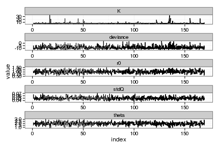
Convergence diagnostics for parametric bayes
tmp <- lapply(as.mcmc(myers_jags), as.matrix) # strip classes
myers_posteriors <- melt(tmp, id = colnames(tmp[[1]]))
names(myers_posteriors) = c("index", "variable", "value", "chain")
ggplot(myers_posteriors) + geom_line(aes(index, value)) +
  facet_wrap(~ variable, scale="free", ncol=1)
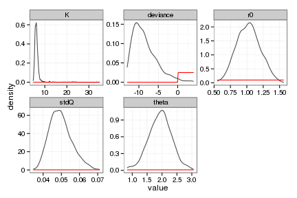
par_prior_curves <- ddply(myers_posteriors, "variable", function(dd){
    grid <- seq(min(dd$value), max(dd$value), length = 100)
    data.frame(value = grid, density = par_priors[[dd$variable[1]]](grid))
})

ggplot(myers_posteriors, aes(value)) +
  stat_density(geom="path", position="identity", alpha=0.7) +
  geom_line(data=par_prior_curves, aes(x=value, y=density), col="red") +
  facet_wrap(~ variable, scale="free", ncol=3)
A <- myers_posteriors
A$index <- A$index + A$chain * max(A$index) # Combine samples across chains by renumbering index
myers_pardist <- acast(A, index ~ variable)
bayes_coef <- apply(myers_pardist,2, posterior.mode) # much better estimates
myers_bayes_pars <- unname(c(bayes_coef[2], bayes_coef[3], bayes_coef[1]))
myers_means <- sapply(x_grid, Myer_harvest, 0, myers_bayes_pars)
myers_f <- function(x,h,p) Myer_harvest(x, h, p[c("r0", "theta", "K")])
head(myers_pardist)
        K deviance     r0    stdQ theta
170 5.444  -11.950 1.0954 0.04771 1.879
171 5.791  -11.106 1.0380 0.04859 1.939
172 6.866  -10.293 0.7794 0.04780 2.390
173 6.454   -8.193 0.9440 0.05598 1.942
174 6.509  -10.105 0.8041 0.04375 2.444
175 7.039   -9.427 0.7927 0.04561 2.297
myers_bayes_pars
[1] -10.158 1.001 5.891
Phase-space diagram of the expected dynamics
models <- data.frame(x=x_grid,
                                         GP=tgp_dat$y,
                                         True=true_means,
                     MLE=est_means,
                                         Ricker=ricker_means,
                     Allen = allen_means,
                     Myers = myers_means)
models <- melt(models, id="x")

# some labels
names(models) <- c("x", "method", "value")

# labels for the colorkey too
model_names = c("GP", "True", "MLE", "Ricker", "Allen", "Myers")
colorkey=cbPalette
names(colorkey) = model_names
plot_gp <- ggplot(tgp_dat) + geom_ribbon(aes(x,y,ymin=ymin,ymax=ymax), fill="gray80") +
    geom_line(data=models, aes(x, value, col=method), lwd=1, alpha=0.8) +
    geom_point(data=obs, aes(x,y), alpha=0.8) +
    xlab(expression(X[t])) + ylab(expression(X[t+1])) +
    scale_colour_manual(values=cbPalette)
print(plot_gp)
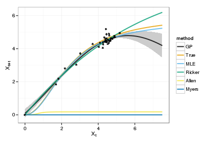
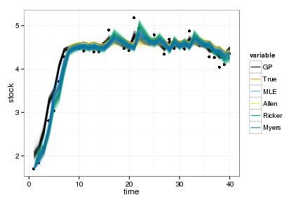
Goodness of fit
This shows only the mean predictions. For the Bayesian cases, we can instead loop over the posteriors of the parameters (or samples from the GP posterior) to get the distribution of such curves in each case.
require(MASS)
step_ahead <- function(x, f, p){
  h = 0
  x_predict <- sapply(x, f, h, p)
  n <- length(x_predict) - 1
  y <- c(x[1], x_predict[1:n])
  y
}
step_ahead_posteriors <- function(x){
gp_f_at_obs <- gp_predict(gp, x, burnin=1e4, thin=300)
df_post <- melt(lapply(sample(100),
  function(i){
    data.frame(time = 1:length(x), stock = x,
                GP = mvrnorm(1, gp_f_at_obs$Ef_posterior[,i], gp_f_at_obs$Cf_posterior[[i]]),
                True = step_ahead(x,f,p),
                MLE = step_ahead(x,f,est$p),
                Allen = step_ahead(x, allen_f, pardist[i,]),
                Ricker = step_ahead(x, ricker_f, ricker_pardist[i,]),
                Myers = step_ahead(x, myers_f, myers_pardist[i,]))
  }), id=c("time", "stock"))
}

df_post <- step_ahead_posteriors(x)

ggplot(df_post) + geom_point(aes(time, stock)) +
  geom_line(aes(time, value, col=variable, group=interaction(L1,variable)), alpha=.1) +
  scale_colour_manual(values=colorkey, guide = guide_legend(override.aes = list(alpha = 1)))
Optimal policies by value iteration
Compute the optimal policy under each model using stochastic dynamic programming. We begin with the policy based on the GP model,
MaxT = 1000
# uses expected values from GP, instead of integrating over posterior
#matrices_gp <- gp_transition_matrix(gp_dat$E_Ef, gp_dat$E_Vf, x_grid, h_grid)

# Integrate over posteriors
matrices_gp <- gp_transition_matrix(gp_dat$Ef_posterior, gp_dat$Vf_posterior, x_grid, h_grid)

# Solve the SDP using the GP-derived transition matrix
opt_gp <- value_iteration(matrices_gp, x_grid, h_grid, MaxT, xT, profit, delta, reward)
Determine the optimal policy based on the allen and MLE models
matrices_true <- f_transition_matrix(f, p, x_grid, h_grid, sigma_g)
opt_true <- value_iteration(matrices_true, x_grid, h_grid, OptTime=MaxT, xT, profit, delta=delta)

matrices_estimated <- f_transition_matrix(est$f, est$p, x_grid, h_grid, est$sigma_g)
opt_estimated <- value_iteration(matrices_estimated, x_grid, h_grid, OptTime=MaxT, xT, profit, delta=delta)
Determine the optimal policy based on Bayesian Allen model
matrices_allen <- parameter_uncertainty_SDP(allen_f, x_grid, h_grid, pardist, 4)
opt_allen <- value_iteration(matrices_allen, x_grid, h_grid, OptTime=MaxT, xT, profit, delta=delta)
Bayesian Ricker
matrices_ricker <- parameter_uncertainty_SDP(ricker_f, x_grid, h_grid, as.matrix(ricker_pardist), 3)
opt_ricker <- value_iteration(matrices_ricker, x_grid, h_grid, OptTime=MaxT, xT, profit, delta=delta)
Bayesian Myers model
matrices_myers <- parameter_uncertainty_SDP(myers_f, x_grid, h_grid, as.matrix(myers_pardist), 4)
myers_alt <- value_iteration(matrices_myers, x_grid, h_grid, OptTime=MaxT, xT, profit, delta=delta)
Assemble the data
OPT = data.frame(GP = opt_gp$D, True = opt_true$D, MLE = opt_estimated$D, Ricker = opt_ricker$D, Allen = opt_allen$D, Myers = myers_alt$D)
colorkey=cbPalette
names(colorkey) = names(OPT)
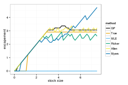
Graph of the optimal policies
policies <- melt(data.frame(stock=x_grid, sapply(OPT, function(x) x_grid[x])), id="stock")
names(policies) <- c("stock", "method", "value")

ggplot(policies, aes(stock, stock - value, color=method)) +
  geom_line(lwd=1.2, alpha=0.8) + xlab("stock size") + ylab("escapement")  +
  scale_colour_manual(values=colorkey)
Simulate 100 realizations managed under each of the policies
sims <- lapply(OPT, function(D){
  set.seed(1)
  lapply(1:100, function(i)
    ForwardSimulate(f, p, x_grid, h_grid, x0, D, z_g, profit=profit, OptTime=OptTime)
  )
})

dat <- melt(sims, id=names(sims[[1]][[1]]))
dt <- data.table(dat)
setnames(dt, c("L1", "L2"), c("method", "reps"))
# Legend in original ordering please, not alphabetical:
dt$method = factor(dt$method, ordered=TRUE, levels=names(OPT))
ggplot(dt) +
  geom_line(aes(time, fishstock, group=interaction(reps,method), color=method), alpha=.1) +
  scale_colour_manual(values=colorkey, guide = guide_legend(override.aes = list(alpha = 1)))
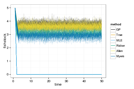
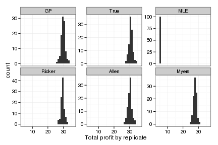
Profit <- dt[, sum(profit), by=c("reps", "method")]
Profit[, mean(V1), by="method"]
   method    V1
1:     GP 30.06
2:   True 31.14
3:    MLE  5.00
4: Ricker 29.82
5:  Allen 30.53
6:  Myers 27.93
ggplot(Profit, aes(V1)) + geom_histogram() +
  facet_wrap(~method, scales = "free_y") + guides(legend.position = "none") + xlab("Total profit by replicate")
allen_deviance <- posterior.mode(pardist[,'deviance'])
ricker_deviance <- posterior.mode(ricker_pardist[,'deviance'])
myers_deviance <- posterior.mode(myers_pardist[,'deviance'])
true_deviance <- 2*estf(c(p, sigma_g))
mle_deviance <- 2*estf(c(est$p, est$sigma_g))

c(allen = allen_deviance, ricker=ricker_deviance, myers=myers_deviance, true=true_deviance, mle=mle_deviance)
     allen     ricker      myers       true        mle
    -7.529     -2.893    -10.158   -106.638 -16204.252
cboettig/nonparametric-bayes documentation built on May 13, 2019, 2:09 p.m.
R Package Documentation
Browse R Packages
We want your feedback!
Note that we can't provide technical support on individual packages. You should contact the package authors for that.
Comparison of Nonparametric Bayesian Gaussian Process estimates to standard the Parametric Bayesian approach
Plotting and knitr options, (can generally be ignored)
require(modeest)
posterior.mode <- function(x) {
mlv(x, method="shorth")$M
}
Model and parameters
f <- Myers
p <- c(1, 2, 6)
K <- 5 # approx, a li'l' less
allee <- 1.2 # approx, a li'l' less
Various parameters defining noise dynamics, grid, and policy costs.
sigma_g <- 0.05
sigma_m <- 0.0
z_g <- function() rlnorm(1, 0, sigma_g)
z_m <- function() 1+(2*runif(1, 0, 1)-1) * sigma_m
x_grid <- seq(0, 1.5 * K, length=50)
h_grid <- x_grid
profit <- function(x,h) pmin(x, h)
delta <- 0.01
OptTime <- 50 # stationarity with unstable models is tricky thing
reward <- 0
xT <- 0
Xo <- allee+.5# observations start from
x0 <- K # simulation under policy starts from
Tobs <- 40
Sample Data
set.seed(1234)
#harvest <- sort(rep(seq(0, .5, length=7), 5))
x <- numeric(Tobs)
x[1] <- Xo
nz <- 1
for(t in 1:(Tobs-1))
x[t+1] = z_g() * f(x[t], h=0, p=p)
obs <- data.frame(x = c(rep(0,nz),
pmax(rep(0,Tobs-1), x[1:(Tobs-1)])),
y = c(rep(0,nz),
x[2:Tobs]))
raw_plot <- ggplot(data.frame(time = 1:Tobs, x=x), aes(time,x)) + geom_line()
raw_plot
Maximum Likelihood
set.seed(12345)
estf <- function(p){
mu <- f(obs$x,0,p)
-sum(dlnorm(obs$y, log(mu), p[4]), log=TRUE)
}
par <- c(p[1]*rlnorm(1,0,.2),
p[2]*rlnorm(1,0,.1),
p[3]*rlnorm(1,0, .1),
sigma_g * rlnorm(1,0,.3))
o <- optim(par, estf, method="L", lower=c(1e-5,1e-5,1e-5,1e-5))
f_alt <- f
p_alt <- c(as.numeric(o$par[1]), as.numeric(o$par[2]), as.numeric(o$par[3]))
sigma_g_alt <- as.numeric(o$par[4])
est <- list(f = f_alt, p = p_alt, sigma_g = sigma_g_alt, mloglik=o$value)
Mean predictions
true_means <- sapply(x_grid, f, 0, p)
est_means <- sapply(x_grid, est$f, 0, est$p)
Non-parametric Bayes
#inv gamma has mean b / (a - 1) (assuming a>1) and variance b ^ 2 / ((a - 2) * (a - 1) ^ 2) (assuming a>2)
s2.p <- c(5,5)
d.p = c(10, 1/0.1)
Estimate the Gaussian Process (nonparametric Bayesian fit)
gp <- gp_mcmc(obs$x, y=obs$y, n=1e5, s2.p = s2.p, d.p = d.p)
gp_dat <- gp_predict(gp, x_grid, burnin=1e4, thin=300)
Show traces and posteriors against priors
plots <- summary_gp_mcmc(gp, burnin=1e4, thin=300)
# Summarize the GP model
tgp_dat <-
data.frame( x = x_grid,
y = gp_dat$E_Ef,
ymin = gp_dat$E_Ef - 2 * sqrt(gp_dat$E_Vf),
ymax = gp_dat$E_Ef + 2 * sqrt(gp_dat$E_Vf) )
Parametric Bayesian Models
We use the JAGS Gibbs sampler, a recent open source BUGS
implementation with an R interface that works on most platforms.
We initialize the usual MCMC parameters; see ?jags for details.
All parametric Bayesian estimates use the following basic parameters for the JAGS MCMC:
y <- x
N <- length(x);
jags.data <- list("N","y")
n.chains <- 6
n.iter <- 1e6
n.burnin <- floor(10000)
n.thin <- max(1, floor(n.chains * (n.iter - n.burnin)/1000))
n.update <- 10
We will use the same priors for process and observation noise in each model,
stdQ_prior_p <- c(1e-6, 100)
stdR_prior_p <- c(1e-6, .1)
stdQ_prior <- function(x) dunif(x, stdQ_prior_p[1], stdQ_prior_p[2])
stdR_prior <- function(x) dunif(x, stdR_prior_p[1], stdR_prior_p[2])
Parametric Bayes of correct (Allen) model
We initiate the MCMC chain (init_p) using the true values of the
parameters p from the simulation. While impossible in real data, this
gives the parametric Bayesian approach the best chance at succeeding.
y is the timeseries (recall obs has the $x_t$, $x_{t+1}$ pairs)
The actual model is defined in a model.file that contains an R function
that is automatically translated into BUGS code by R2WinBUGS. The file
defines the priors and the model. We write the file from R as follows:
K_prior_p <- c(0.01, 20.0)
r0_prior_p <- c(0.01, 6.0)
theta_prior_p <- c(0.01, 20.0)
bugs.model <-
paste(sprintf(
"model{
K ~ dunif(%s, %s)
r0 ~ dunif(%s, %s)
theta ~ dunif(%s, %s)
stdQ ~ dunif(%s, %s)",
K_prior_p[1], K_prior_p[2],
r0_prior_p[1], r0_prior_p[2],
theta_prior_p[1], theta_prior_p[2],
stdQ_prior_p[1], stdQ_prior_p[2]),
"
iQ <- 1 / (stdQ * stdQ);
y[1] ~ dunif(0, 10)
for(t in 1:(N-1)){
mu[t] <- log(y[t]) + r0 * (1 - y[t]/K)* (y[t] - theta) / K
y[t+1] ~ dlnorm(mu[t], iQ)
}
}")
writeLines(bugs.model, "allen_process.bugs")
Write the priors into a list for later reference
K_prior <- function(x) dunif(x, K_prior_p[1], K_prior_p[2])
r0_prior <- function(x) dunif(x, r0_prior_p[1], r0_prior_p[2])
theta_prior <- function(x) dunif(x, theta_prior_p[1], theta_prior_p[2])
par_priors <- list(K = K_prior, deviance = function(x) 0 * x,
r0 = r0_prior, theta = theta_prior,
stdQ = stdQ_prior)
We define which parameters to keep track of, and set the initial values of parameters in the transformed space used by the MCMC. We use logarithms to maintain strictly positive values of parameters where appropriate.
jags.params=c("K","r0","theta","stdQ") # be sensible about the order here
jags.inits <- function(){
list("K"= 8 * rlnorm(1,0, 0.1),
"r0"= 2 * rlnorm(1,0, 0.1) ,
"theta"= 5 * rlnorm(1,0, 0.1) ,
"stdQ"= abs( 0.1 * rlnorm(1,0, 0.1)),
.RNG.name="base::Wichmann-Hill", .RNG.seed=123)
}
set.seed(1234)
# parallel refuses to take variables as arguments (e.g. n.iter = 1e5 works, but n.iter = n doesn't)
allen_jags <- do.call(jags.parallel, list(data=jags.data, inits=jags.inits,
jags.params, n.chains=n.chains,
n.iter=n.iter, n.thin=n.thin,
n.burnin=n.burnin,
model.file="allen_process.bugs"))
# Run again iteratively if we haven't met the Gelman-Rubin convergence criterion
recompile(allen_jags) # required for parallel
allen_jags <- do.call(autojags,
list(object=allen_jags, n.update=n.update,
n.iter=n.iter, n.thin = n.thin))
Convergence diagnostics for Allen model
R notes: this strips classes from the mcmc.list object (so that we have list of matrices; objects that reshape2::melt can handle intelligently), and then combines chains into one array. In this array each parameter is given its value at each sample from the posterior (index) for each chain.
tmp <- lapply(as.mcmc(allen_jags), as.matrix) # strip classes the hard way...
allen_posteriors <- melt(tmp, id = colnames(tmp[[1]]))
names(allen_posteriors) = c("index", "variable", "value", "chain")
ggplot(allen_posteriors) + geom_line(aes(index, value)) +
facet_wrap(~ variable, scale="free", ncol=1)
allen_priors <- ddply(allen_posteriors, "variable", function(dd){
grid <- seq(min(dd$value), max(dd$value), length = 100)
data.frame(value = grid, density = par_priors[[dd$variable[1]]](grid))
})
ggplot(allen_posteriors, aes(value)) +
stat_density(geom="path", position="identity", alpha=0.7) +
geom_line(data=allen_priors, aes(x=value, y=density), col="red") +
facet_wrap(~ variable, scale="free", ncol=3)
Reshape the posterior parameter distribution data, transform back into original space, and calculate the mean parameters and mean function
A <- allen_posteriors
A$index <- A$index + A$chain * max(A$index) # Combine samples across chains by renumbering index
pardist <- acast(A, index ~ variable)
bayes_coef <- apply(pardist,2, posterior.mode)
bayes_pars <- unname(c(bayes_coef["r0"], bayes_coef["K"], bayes_coef["theta"])) # parameters formatted for f
allen_f <- function(x,h,p) unname(RickerAllee(x,h, unname(p[c("r0", "K", "theta")])))
allen_means <- sapply(x_grid, f, 0, bayes_pars)
bayes_pars
[1] 0.7082 4.5647 0.2558
head(pardist)
K deviance r0 stdQ theta
170 4.531 -8.534 0.6867 0.04473 0.3832
171 4.516 1.335 0.6471 0.05928 1.0216
172 4.574 -8.576 0.8532 0.04983 0.7196
173 4.614 -6.873 0.5302 0.04611 0.1390
174 4.628 -5.580 0.7331 0.04024 0.5064
175 4.503 -7.443 0.7341 0.04474 0.2369
Parametric Bayes based on the structurally wrong model (Ricker)
K_prior_p <- c(0.01, 40.0)
r0_prior_p <- c(0.01, 20.0)
bugs.model <-
paste(sprintf(
"model{
K ~ dunif(%s, %s)
r0 ~ dunif(%s, %s)
stdQ ~ dunif(%s, %s)",
K_prior_p[1], K_prior_p[2],
r0_prior_p[1], r0_prior_p[2],
stdQ_prior_p[1], stdQ_prior_p[2]),
"
iQ <- 1 / (stdQ * stdQ);
y[1] ~ dunif(0, 10)
for(t in 1:(N-1)){
mu[t] <- log(y[t]) + r0 * (1 - y[t]/K)
y[t+1] ~ dlnorm(mu[t], iQ)
}
}")
writeLines(bugs.model, "ricker_process.bugs")
Compute prior curves
K_prior <- function(x) dunif(x, K_prior_p[1], K_prior_p[2])
r0_prior <- function(x) dunif(x, r0_prior_p[1], r0_prior_p[2])
par_priors <- list(K = K_prior, deviance = function(x) 0 * x,
r0 = r0_prior, stdQ = stdQ_prior)
We define which parameters to keep track of, and set the initial values of parameters in the transformed space used by the MCMC.
jags.params=c("K","r0", "stdQ")
jags.inits <- function(){
list("K"=10 * rlnorm(1,0,.5),
"r0"= rlnorm(1,0,.5),
"stdQ"=sqrt(0.05) * rlnorm(1,0,.5),
.RNG.name="base::Wichmann-Hill", .RNG.seed=123)
}
set.seed(12345)
ricker_jags <- do.call(jags.parallel,
list(data=jags.data, inits=jags.inits,
jags.params, n.chains=n.chains,
n.iter=n.iter, n.thin=n.thin, n.burnin=n.burnin,
model.file="ricker_process.bugs"))
recompile(ricker_jags)
Compiling model graph
Resolving undeclared variables
Allocating nodes
Graph Size: 249
Initializing model
Compiling model graph
Resolving undeclared variables
Allocating nodes
Graph Size: 249
Initializing model
Compiling model graph
Resolving undeclared variables
Allocating nodes
Graph Size: 249
Initializing model
Compiling model graph
Resolving undeclared variables
Allocating nodes
Graph Size: 249
Initializing model
Compiling model graph
Resolving undeclared variables
Allocating nodes
Graph Size: 249
Initializing model
Compiling model graph
Resolving undeclared variables
Allocating nodes
Graph Size: 249
Initializing model
ricker_jags <- do.call(autojags,
list(object=ricker_jags, n.update=n.update,
n.iter=n.iter, n.thin = n.thin,
progress.bar="none"))
Convergence diagnostics for parametric bayes Ricker model
tmp <- lapply(as.mcmc(ricker_jags), as.matrix) # strip classes the hard way...
ricker_posteriors <- melt(tmp, id = colnames(tmp[[1]]))
names(ricker_posteriors) = c("index", "variable", "value", "chain")
ggplot(ricker_posteriors) + geom_line(aes(index, value)) +
facet_wrap(~ variable, scale="free", ncol=1)
ricker_priors <- ddply(ricker_posteriors, "variable", function(dd){
grid <- seq(min(dd$value), max(dd$value), length = 100)
data.frame(value = grid, density = par_priors[[dd$variable[1]]](grid))
})
# plot posterior distributions
ggplot(ricker_posteriors, aes(value)) +
stat_density(geom="path", position="identity", alpha=0.7) +
geom_line(data=ricker_priors, aes(x=value, y=density), col="red") +
facet_wrap(~ variable, scale="free", ncol=2)
Reshape posteriors data, transform back, calculate mode and corresponding function.
A <- ricker_posteriors
A$index <- A$index + A$chain * max(A$index) # Combine samples across chains by renumbering index
ricker_pardist <- acast(A, index ~ variable)
bayes_coef <- apply(ricker_pardist,2, posterior.mode)
ricker_bayes_pars <- unname(c(bayes_coef["r0"], bayes_coef["K"]))
ricker_f <- function(x,h,p){
sapply(x, function(x){
x <- pmax(0, x-h)
pmax(0, x * exp(p["r0"] * (1 - x / p["K"] )) )
})
}
ricker_means <- sapply(x_grid, Ricker, 0, ricker_bayes_pars[c(1,2)])
head(ricker_pardist)
K deviance r0 stdQ
170 4.796 -2.4558 0.2928 0.05125
171 4.604 4.2228 0.4464 0.06022
172 4.579 -3.6943 0.2798 0.05368
173 4.727 0.8348 0.2275 0.06162
174 4.686 0.1420 0.2346 0.04685
175 4.361 -0.5967 0.2783 0.05220
ricker_bayes_pars
[1] 0.302 4.597
Myers Parametric Bayes
r0_prior_p <- c(.0001, 10.0)
theta_prior_p <- c(.0001, 10.0)
K_prior_p <- c(.0001, 40.0)
bugs.model <-
paste(sprintf(
"model{
r0 ~ dunif(%s, %s)
theta ~ dunif(%s, %s)
K ~ dunif(%s, %s)
stdQ ~ dunif(%s, %s)",
r0_prior_p[1], r0_prior_p[2],
theta_prior_p[1], theta_prior_p[2],
K_prior_p[1], K_prior_p[2],
stdQ_prior_p[1], stdQ_prior_p[2]),
"
iQ <- 1 / (stdQ * stdQ);
y[1] ~ dunif(0, 10)
for(t in 1:(N-1)){
mu[t] <- log(r0) + theta * log(y[t]) - log(1 + pow(abs(y[t]), theta) / K)
y[t+1] ~ dlnorm(mu[t], iQ)
}
}")
writeLines(bugs.model, "myers_process.bugs")
K_prior <- function(x) dunif(x, K_prior_p[1], K_prior_p[2])
r_prior <- function(x) dunif(x, r0_prior_p[1], r0_prior_p[2])
theta_prior <- function(x) dunif(x, theta_prior_p[1], theta_prior_p[2])
par_priors <- list( deviance = function(x) 0 * x, K = K_prior,
r0 = r_prior, theta = theta_prior,
stdQ = stdQ_prior)
jags.params=c("r0", "theta", "K", "stdQ")
jags.inits <- function(){
list("r0"= rlnorm(1,0,.1),
"K"= 6 * rlnorm(1,0,.1),
"theta" = 2 * rlnorm(1,0,.1),
"stdQ"= 0.1 * rlnorm(1,0,.1),
.RNG.name="base::Wichmann-Hill", .RNG.seed=123)
}
set.seed(12345)
myers_jags <- do.call(jags.parallel,
list(data=jags.data, inits=jags.inits,
jags.params, n.chains=n.chains,
n.iter=n.iter, n.thin=n.thin,
n.burnin=n.burnin,
model.file="myers_process.bugs"))
recompile(myers_jags)
Compiling model graph
Resolving undeclared variables
Allocating nodes
Graph Size: 406
Initializing model
Compiling model graph
Resolving undeclared variables
Allocating nodes
Graph Size: 406
Initializing model
Compiling model graph
Resolving undeclared variables
Allocating nodes
Graph Size: 406
Initializing model
Compiling model graph
Resolving undeclared variables
Allocating nodes
Graph Size: 406
Initializing model
Compiling model graph
Resolving undeclared variables
Allocating nodes
Graph Size: 406
Initializing model
Compiling model graph
Resolving undeclared variables
Allocating nodes
Graph Size: 406
Initializing model
myers_jags <- do.call(autojags,
list(myers_jags, n.update=n.update,
n.iter=n.iter, n.thin = n.thin,
progress.bar="none"))
Convergence diagnostics for parametric bayes
tmp <- lapply(as.mcmc(myers_jags), as.matrix) # strip classes
myers_posteriors <- melt(tmp, id = colnames(tmp[[1]]))
names(myers_posteriors) = c("index", "variable", "value", "chain")
ggplot(myers_posteriors) + geom_line(aes(index, value)) +
facet_wrap(~ variable, scale="free", ncol=1)
par_prior_curves <- ddply(myers_posteriors, "variable", function(dd){
grid <- seq(min(dd$value), max(dd$value), length = 100)
data.frame(value = grid, density = par_priors[[dd$variable[1]]](grid))
})
ggplot(myers_posteriors, aes(value)) +
stat_density(geom="path", position="identity", alpha=0.7) +
geom_line(data=par_prior_curves, aes(x=value, y=density), col="red") +
facet_wrap(~ variable, scale="free", ncol=3)
A <- myers_posteriors
A$index <- A$index + A$chain * max(A$index) # Combine samples across chains by renumbering index
myers_pardist <- acast(A, index ~ variable)
bayes_coef <- apply(myers_pardist,2, posterior.mode) # much better estimates
myers_bayes_pars <- unname(c(bayes_coef[2], bayes_coef[3], bayes_coef[1]))
myers_means <- sapply(x_grid, Myer_harvest, 0, myers_bayes_pars)
myers_f <- function(x,h,p) Myer_harvest(x, h, p[c("r0", "theta", "K")])
head(myers_pardist)
K deviance r0 stdQ theta
170 5.444 -11.950 1.0954 0.04771 1.879
171 5.791 -11.106 1.0380 0.04859 1.939
172 6.866 -10.293 0.7794 0.04780 2.390
173 6.454 -8.193 0.9440 0.05598 1.942
174 6.509 -10.105 0.8041 0.04375 2.444
175 7.039 -9.427 0.7927 0.04561 2.297
myers_bayes_pars
[1] -10.158 1.001 5.891
Phase-space diagram of the expected dynamics
models <- data.frame(x=x_grid,
GP=tgp_dat$y,
True=true_means,
MLE=est_means,
Ricker=ricker_means,
Allen = allen_means,
Myers = myers_means)
models <- melt(models, id="x")
# some labels
names(models) <- c("x", "method", "value")
# labels for the colorkey too
model_names = c("GP", "True", "MLE", "Ricker", "Allen", "Myers")
colorkey=cbPalette
names(colorkey) = model_names
plot_gp <- ggplot(tgp_dat) + geom_ribbon(aes(x,y,ymin=ymin,ymax=ymax), fill="gray80") +
geom_line(data=models, aes(x, value, col=method), lwd=1, alpha=0.8) +
geom_point(data=obs, aes(x,y), alpha=0.8) +
xlab(expression(X[t])) + ylab(expression(X[t+1])) +
scale_colour_manual(values=cbPalette)
print(plot_gp)
Goodness of fit
This shows only the mean predictions. For the Bayesian cases, we can instead loop over the posteriors of the parameters (or samples from the GP posterior) to get the distribution of such curves in each case.
require(MASS)
step_ahead <- function(x, f, p){
h = 0
x_predict <- sapply(x, f, h, p)
n <- length(x_predict) - 1
y <- c(x[1], x_predict[1:n])
y
}
step_ahead_posteriors <- function(x){
gp_f_at_obs <- gp_predict(gp, x, burnin=1e4, thin=300)
df_post <- melt(lapply(sample(100),
function(i){
data.frame(time = 1:length(x), stock = x,
GP = mvrnorm(1, gp_f_at_obs$Ef_posterior[,i], gp_f_at_obs$Cf_posterior[[i]]),
True = step_ahead(x,f,p),
MLE = step_ahead(x,f,est$p),
Allen = step_ahead(x, allen_f, pardist[i,]),
Ricker = step_ahead(x, ricker_f, ricker_pardist[i,]),
Myers = step_ahead(x, myers_f, myers_pardist[i,]))
}), id=c("time", "stock"))
}
df_post <- step_ahead_posteriors(x)
ggplot(df_post) + geom_point(aes(time, stock)) +
geom_line(aes(time, value, col=variable, group=interaction(L1,variable)), alpha=.1) +
scale_colour_manual(values=colorkey, guide = guide_legend(override.aes = list(alpha = 1)))
Optimal policies by value iteration
Compute the optimal policy under each model using stochastic dynamic programming. We begin with the policy based on the GP model,
MaxT = 1000
# uses expected values from GP, instead of integrating over posterior
#matrices_gp <- gp_transition_matrix(gp_dat$E_Ef, gp_dat$E_Vf, x_grid, h_grid)
# Integrate over posteriors
matrices_gp <- gp_transition_matrix(gp_dat$Ef_posterior, gp_dat$Vf_posterior, x_grid, h_grid)
# Solve the SDP using the GP-derived transition matrix
opt_gp <- value_iteration(matrices_gp, x_grid, h_grid, MaxT, xT, profit, delta, reward)
Determine the optimal policy based on the allen and MLE models
matrices_true <- f_transition_matrix(f, p, x_grid, h_grid, sigma_g)
opt_true <- value_iteration(matrices_true, x_grid, h_grid, OptTime=MaxT, xT, profit, delta=delta)
matrices_estimated <- f_transition_matrix(est$f, est$p, x_grid, h_grid, est$sigma_g)
opt_estimated <- value_iteration(matrices_estimated, x_grid, h_grid, OptTime=MaxT, xT, profit, delta=delta)
Determine the optimal policy based on Bayesian Allen model
matrices_allen <- parameter_uncertainty_SDP(allen_f, x_grid, h_grid, pardist, 4)
opt_allen <- value_iteration(matrices_allen, x_grid, h_grid, OptTime=MaxT, xT, profit, delta=delta)
Bayesian Ricker
matrices_ricker <- parameter_uncertainty_SDP(ricker_f, x_grid, h_grid, as.matrix(ricker_pardist), 3)
opt_ricker <- value_iteration(matrices_ricker, x_grid, h_grid, OptTime=MaxT, xT, profit, delta=delta)
Bayesian Myers model
matrices_myers <- parameter_uncertainty_SDP(myers_f, x_grid, h_grid, as.matrix(myers_pardist), 4)
myers_alt <- value_iteration(matrices_myers, x_grid, h_grid, OptTime=MaxT, xT, profit, delta=delta)
Assemble the data
OPT = data.frame(GP = opt_gp$D, True = opt_true$D, MLE = opt_estimated$D, Ricker = opt_ricker$D, Allen = opt_allen$D, Myers = myers_alt$D)
colorkey=cbPalette
names(colorkey) = names(OPT)
Graph of the optimal policies
policies <- melt(data.frame(stock=x_grid, sapply(OPT, function(x) x_grid[x])), id="stock")
names(policies) <- c("stock", "method", "value")
ggplot(policies, aes(stock, stock - value, color=method)) +
geom_line(lwd=1.2, alpha=0.8) + xlab("stock size") + ylab("escapement") +
scale_colour_manual(values=colorkey)
Simulate 100 realizations managed under each of the policies
sims <- lapply(OPT, function(D){
set.seed(1)
lapply(1:100, function(i)
ForwardSimulate(f, p, x_grid, h_grid, x0, D, z_g, profit=profit, OptTime=OptTime)
)
})
dat <- melt(sims, id=names(sims[[1]][[1]]))
dt <- data.table(dat)
setnames(dt, c("L1", "L2"), c("method", "reps"))
# Legend in original ordering please, not alphabetical:
dt$method = factor(dt$method, ordered=TRUE, levels=names(OPT))
ggplot(dt) +
geom_line(aes(time, fishstock, group=interaction(reps,method), color=method), alpha=.1) +
scale_colour_manual(values=colorkey, guide = guide_legend(override.aes = list(alpha = 1)))
Profit <- dt[, sum(profit), by=c("reps", "method")]
Profit[, mean(V1), by="method"]
method V1
1: GP 30.06
2: True 31.14
3: MLE 5.00
4: Ricker 29.82
5: Allen 30.53
6: Myers 27.93
ggplot(Profit, aes(V1)) + geom_histogram() +
facet_wrap(~method, scales = "free_y") + guides(legend.position = "none") + xlab("Total profit by replicate")
allen_deviance <- posterior.mode(pardist[,'deviance'])
ricker_deviance <- posterior.mode(ricker_pardist[,'deviance'])
myers_deviance <- posterior.mode(myers_pardist[,'deviance'])
true_deviance <- 2*estf(c(p, sigma_g))
mle_deviance <- 2*estf(c(est$p, est$sigma_g))
c(allen = allen_deviance, ricker=ricker_deviance, myers=myers_deviance, true=true_deviance, mle=mle_deviance)
allen ricker myers true mle
-7.529 -2.893 -10.158 -106.638 -16204.252
R Package Documentation
Browse R Packages
We want your feedback!
Note that we can't provide technical support on individual packages. You should contact the package authors for that.
Embedding an R snippet on your website
Add the following code to your website.
For more information on customizing the embed code, read Embedding Snippets.