inst/examples/BUGS/policy_thresholds.md
In cboettig/nonparametric-bayes: Nonparametric Bayes inference for ecological models
Comparison of Nonparametric Bayesian Gaussian Process estimates to standard the Parametric Bayesian approach
setwd("~/Documents/code/nonparametric-bayes/inst/examples/BUGS/")
Plotting and knitr options, (can generally be ignored)
library(knitcitations)
## Loading required package: bibtex
opts_chunk$set(tidy = FALSE, warning = FALSE, message = FALSE, cache = FALSE,
    comment = NA, fig.width = 6, fig.height = 4)

library(ggplot2)  # plotting
opts_knit$set(upload.fun = socialR::flickr.url)
theme_set(theme_bw(base_size = 10))
theme_update(panel.background = element_rect(fill = "transparent", colour = NA),
    plot.background = element_rect(fill = "transparent", colour = NA))
cbPalette <- c("#000000", "#E69F00", "#56B4E9", "#009E73", "#F0E442", "#0072B2",
    "#D55E00", "#CC79A7")
Load necessary libraries,
library(nonparametricbayes) # loads the rest as dependencies
Model and parameters
Uses the model derived in citet("10.1080/10236190412331335373"), of a Ricker-like growth curve with an allee effect, defined in the pdgControl package,
f <- Ricker
p <- c(1, 10)
K <- p[2]
C <- 5 # policy threshold
Various parameters defining noise dynamics, grid, and policy costs.
sigma_g <- 0.05
sigma_m <- 0.0
z_g <- function() rlnorm(1, 0, sigma_g)
z_m <- function() 1+(2*runif(1, 0,  1)-1) * sigma_m
x_grid <- seq(0, 1.5 * K, length=50)
h_grid <- x_grid
profit <- function(x,h) pmin(x, h) - 10*(x > C) # big penalty for violating threshold
delta <- 0.01
OptTime <- 50  # stationarity with unstable models is tricky thing
reward <- 0
xT <- 0
Xo <- K # observations start from
x0 <- Xo # simulation under policy starts from
Tobs <- 40
Sample Data
  set.seed(1234)
  #harvest <- sort(rep(seq(0, .5, length=7), 5))
  x <- numeric(Tobs)
  x[1] <- 6
  nz <- 1
  for(t in 1:(Tobs-1))
    x[t+1] = z_g() * f(x[t], h=0, p=p)
  obs <- data.frame(x = c(rep(0,nz),
                          pmax(rep(0,Tobs-1), x[1:(Tobs-1)])),
                    y = c(rep(0,nz),
                          x[2:Tobs]))
# plot(x)
Maximum Likelihood
est <- par_est(obs,  init = c(r = p[1],
                              K = mean(obs$x[obs$x>0]),
                              s = sigma_g))
Non-parametric Bayes
#inv gamma has mean b / (a - 1) (assuming a>1) and variance b ^ 2 / ((a - 2) * (a - 1) ^ 2) (assuming a>2)
s2.p <- c(5,5)
d.p = c(10, 1/0.1)
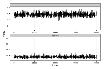
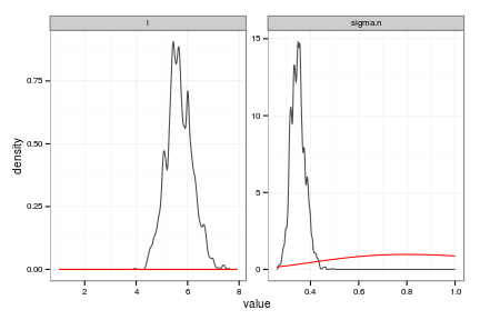
Estimate the Gaussian Process (nonparametric Bayesian fit)
gp <- gp_mcmc(obs$x, y=obs$y, n=1e5, s2.p = s2.p, d.p = d.p)
gp_dat <- gp_predict(gp, x_grid, burnin=1e4, thin=300)
Show traces and posteriors against priors
plots <- summary_gp_mcmc(gp)
# Summarize the GP model
tgp_dat <-
    data.frame(  x = x_grid,
                 y = gp_dat$E_Ef,
                 ymin = gp_dat$E_Ef - 2 * sqrt(gp_dat$E_Vf),
                 ymax = gp_dat$E_Ef + 2 * sqrt(gp_dat$E_Vf) )
Parametric Bayes
We initiate the MCMC chain (init_p) using the true values of the parameters p from the simulation. While impossible in real data, this gives the parametric Bayesian approach the best chance at succeeding. y is the timeseries (recall obs has the $x_t$, $x_{t+1}$ pairs)
# a bit unfair to start with the correct values, but anyhow...
init_p = p
names(init_p) = c("r0", "K", "theta")
Error: 'names' attribute [3] must be the same length as the vector [2]
y <- obs$x[-1]
N=length(y);
We'll be using the JAGS Gibbs sampler, a recent open source BUGS implementation with an R interface that works on most platforms. We initialize the usual MCMC parameters; see ?jags for details.
jags.data <- list("N","y")
n.chains = 1
n.iter = 40000
n.burnin = floor(10000)
n.thin = max(1, floor(n.chains * (n.iter - n.burnin)/1000))
The actual model is defined in a model.file that contains an R function that is automatically translated into BUGS code by R2WinBUGS. The file defines the priors and the model, as seen when read in here
cat(readLines(con="bugmodel-UPrior.txt"), sep="\n")
model{

K     ~ dunif(0.01, 40.0)
logr0    ~ dunif(-6.0, 6.0)
logtheta ~ dunif(-6.0, 6.0)
stdQ ~ dunif(0.0001,100)
stdR ~ dunif(0.0001,100)
# JAGS notation, mean, and precision ( reciprical of the variance, 1/sigma^2)
iQ <- 1/(stdQ*stdQ);
iR <- 1/(stdR*stdR);

r0 <- exp(logr0)
theta <- exp(logtheta)


x[1] ~ dunif(0,10)

for(t in 1:(N-1)){
  mu[t] <- x[t] * exp(r0 * (1 - x[t]/K)* (x[t] - theta) / K )
  x[t+1] ~ dnorm(mu[t],iQ)
}


for(t in 1:(N)){
  y[t] ~ dnorm(x[t],iR)
}

}
We define which parameters to keep track of, and set the initial values of parameters in the transformed space used by the MCMC. We use logarithms to maintain strictly positive values of parameters where appropriate.
# Uniform priors on standard deviation terms
jags.params=c("K","logr0","logtheta","stdQ", "stdR")
jags.inits <- function(){
  list("K"=init_p["K"],"logr0"=log(init_p["r0"]),"logtheta"=log(init_p["theta"]), "stdQ"=sqrt(0.05),"stdR"=sqrt(0.1),"x"=y,.RNG.name="base::Wichmann-Hill", .RNG.seed=123)
}

set.seed(12345)

time_jags <- system.time(
  jagsfit <- jags(data=jags.data, inits=jags.inits, jags.params, n.chains=n.chains,
                  n.iter=n.iter, n.thin=n.thin, n.burnin=n.burnin,model.file="bugmodel-UPrior.txt")
)
Compiling model graph
   Resolving undeclared variables
   Allocating nodes
   Graph Size: 365

Initializing model
time_jags <- unname(time_jags["elapsed"]);
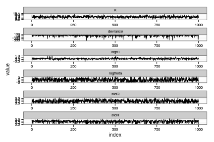
Convergence diagnostics for parametric bayes
jags_matrix <- as.data.frame(as.mcmc.bugs(jagsfit$BUGSoutput))
par_posteriors <- melt(cbind(index = 1:dim(jags_matrix)[1], jags_matrix), id = "index")
# Traces
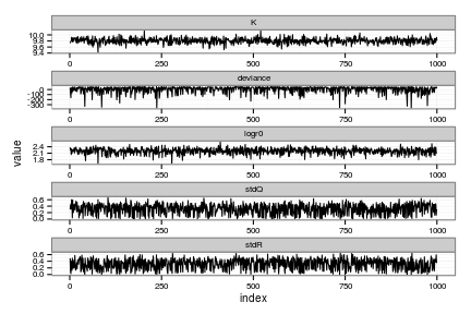
ggplot(par_posteriors) + geom_line(aes(index, value)) + facet_wrap(~ variable, scale="free", ncol=1)
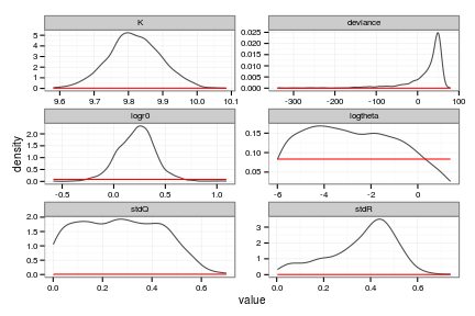
## priors (untransformed variables)
K_prior <- function(x) dunif(x, 0.01, 40)
logr_prior <- function(x) dunif(x, -6, 6)
logtheta_prior <- function(x) dunif(x, -6, 6)
stdQ_prior <- function(x) dunif(x, 0.001, 100)
stdR_prior <- function(x) dunif(x, 0.001, 100)
par_priors <- list(K = K_prior, deviance = function(x) 0 * x,
logr0 = logr_prior, logtheta = logtheta_prior,
stdQ = stdQ_prior, stdR = stdR_prior)
par_prior_curves <- ddply(par_posteriors, "variable", function(dd){
grid <- seq(min(dd$value), max(dd$value), length = 100)
data.frame(value = grid, density = par_priors[[dd$variable[1]]](grid))
})
# posterior distributions
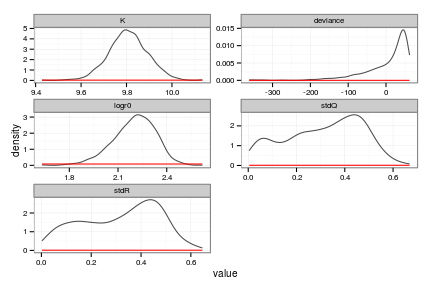
ggplot(par_posteriors, aes(value)) +
stat_density(geom="path", position="identity", alpha=0.7) +
geom_line(data=par_prior_curves, aes(x=value, y=density), col="red") +
facet_wrap(~ variable, scale="free", ncol=2)
# um, cleaner if we were just be using the long form, par_posterior
mcmc <- as.mcmc(jagsfit)
mcmcall <- mcmc[,-2]
who <- colnames(mcmcall)
who
[1] "K" "logr0" "logtheta" "stdQ" "stdR"
mcmcall <- cbind(mcmcall[,1],mcmcall[,2],mcmcall[,3],mcmcall[,4],mcmcall[,5])
colnames(mcmcall) <- who


pardist <- mcmcall
pardist[,2] = exp(pardist[,2]) # transform model parameters back first
pardist[,3] = exp(pardist[,3])


bayes_coef <- apply(pardist,2,mean)
bayes_pars <- unname(c(bayes_coef[2], bayes_coef[1], bayes_coef[3]))
bayes_pars
[1] 1.270 9.818 0.314
par_bayes_means <- sapply(x_grid, f, 0, bayes_pars)
Parametric Bayes based on the structurally wrong model
We initiate the MCMC chain (init_p) using the true values of the parameters p from the simulation. While impossible in real data, this gives the parametric Bayesian approach the best chance at succeeding. y is the timeseries (recall obs has the $x_t$, $x_{t+1}$ pairs)
init_p = p
names(init_p) = c("r0", "K")
y <- obs$x[-1]
N=length(y);
We'll be using the JAGS Gibbs sampler, a recent open source BUGS implementation with an R interface that works on most platforms. We initialize the usual MCMC parameters; see ?jags for details.
jags.data <- list("N","y")
n.chains = 1
n.iter = 40000
n.burnin = floor(10000)
n.thin = max(1, floor(n.chains * (n.iter - n.burnin)/1000))
The actual model is defined in a model.file that contains an R function that is automatically translated into BUGS code by R2WinBUGS. The file defines the priors and the model, as seen when read in here
cat(readLines(con="ricker-UPrior.txt"), sep="\n")
model{

K     ~ dunif(0.01, 40.0)
logr0    ~ dunif(-6.0, 6.0)
stdQ ~ dunif(0.0001,100)
stdR ~ dunif(0.0001,100)
# JAGS notation, mean, and precision ( reciprical of the variance, 1/sigma^2)
iQ <- 1/(stdQ*stdQ);
iR <- 1/(stdR*stdR);

r0 <- exp(logr0)


x[1] ~ dunif(0,10)

for(t in 1:(N-1)){
  mu[t] <- x[t] * exp(r0 * (1 - x[t]/K) / K )
  x[t+1] ~ dnorm(mu[t],iQ)
}


for(t in 1:(N)){
  y[t] ~ dnorm(x[t],iR)
}

}
We define which parameters to keep track of, and set the initial values of parameters in the transformed space used by the MCMC. We use logarithms to maintain strictly positive values of parameters where appropriate.
# Uniform priors on standard deviation terms
jags.params=c("K","logr0", "stdQ", "stdR")
jags.inits <- function(){
  list("K"=init_p["K"],"logr0"=log(init_p["r0"]), "stdQ"=sqrt(0.05),"stdR"=sqrt(0.1),"x"=y,.RNG.name="base::Wichmann-Hill", .RNG.seed=123)
}

set.seed(12345)

time_jags <- system.time(
  jagsfit <- jags(data=jags.data, inits=jags.inits, jags.params, n.chains=n.chains,
                  n.iter=n.iter, n.thin=n.thin, n.burnin=n.burnin,model.file="ricker-UPrior.txt")
)
Compiling model graph
   Resolving undeclared variables
   Allocating nodes
   Graph Size: 325

Initializing model
time_jags <- unname(time_jags["elapsed"]);
Convergence diagnostics for parametric bayes Ricker model
jags_matrix <- as.data.frame(as.mcmc.bugs(jagsfit$BUGSoutput))
par_posteriors <- melt(cbind(index = 1:dim(jags_matrix)[1], jags_matrix), id = "index")

# Traces
ggplot(par_posteriors) + geom_line(aes(index, value)) +
  facet_wrap(~ variable, scale="free", ncol=1)
## priors (untransformed variables)
K_prior <- function(x) dunif(x, 0.01, 40)
logr_prior <- function(x) dunif(x, -6, 6)
stdQ_prior <- function(x) dunif(x, 0.001, 100)
stdR_prior <- function(x) dunif(x, 0.001, 100)

par_priors <- list(K = K_prior, deviance = function(x) 0 * x, logr0 = logr_prior, stdQ = stdQ_prior, stdR = stdR_prior)

par_prior_curves <- ddply(par_posteriors, "variable", function(dd){
    grid <- seq(min(dd$value), max(dd$value), length = 100)
    data.frame(value = grid, density = par_priors[[dd$variable[1]]](grid))
})

# posterior distributions
ggplot(par_posteriors, aes(value)) +
  stat_density(geom="path", position="identity", alpha=0.7) +
  geom_line(data=par_prior_curves, aes(x=value, y=density), col="red") +
  facet_wrap(~ variable, scale="free", ncol=2)
ricker_pardist <- jags_matrix[! names(jags_matrix) == "deviance" ]
ricker_pardist[,"logr0"] = exp(ricker_pardist[,"logr0"]) # transform model parameters back first

posterior.mode <- function(x) {
  ux <- unique(x)
  ux[which.max(tabulate(match(x, ux)))]
}

apply(ricker_pardist,2,mean)
     K  logr0   stdQ   stdR
9.8075 9.0975 0.3128 0.3167
bayes_coef <- apply(ricker_pardist,2, posterior.mode) # much better estimates
ricker_bayes_pars <- unname(c(bayes_coef[2], bayes_coef[1]))
ricker_bayes_pars
[1] 10.73 9.73
Write the external bugs file
logr0_prior_p <- c(-6.0, 6.0)
logtheta_prior_p <- c(-6.0, 6.0)
logK_prior_p <- c(-6.0, 6.0)
stdQ_prior_p <- c(0.0001, 100)
stdR_prior_p <- c(0.0001, 100)

bugs.model <-
paste(sprintf(
"model{
  logr0    ~ dunif(%s, %s)
  logtheta    ~ dunif(%s, %s)
  logK    ~ dunif(%s, %s)
  stdQ ~ dunif(%s, %s)
  stdR ~ dunif(%s, %s)",
  logr0_prior_p[1], logr0_prior_p[2],
  logtheta_prior_p[1], logtheta_prior_p[2],
  logK_prior_p[1], logK_prior_p[2],
  stdQ_prior_p[1], stdQ_prior_p[2],
  stdR_prior_p[1], stdR_prior_p[2]),
  "

  iQ <- 1 / (stdQ * stdQ);
  iR <- 1 / (stdR * stdR);

  r0 <- exp(logr0)
  theta <- exp(logtheta)
  K <- exp(logK)

  x[1] ~ dunif(0, 10)

  for(t in 1:(N-1)){
    mu[t] <- r0 * pow(abs(x[t]), theta) / (1 + pow(abs(x[t]), theta) / K)
    x[t+1] ~ dnorm(mu[t], iQ)
  }

  for(t in 1:(N)){
    y[t] ~ dnorm(x[t], iR)
  }
}")

writeLines(bugs.model, "myers.bugs")
## priors (untransformed variables)
logK_prior     <- function(x) dunif(x, logK_prior_p[1], logK_prior_p[2])
logr_prior     <- function(x) dunif(x, logr0_prior_p[1], logr0_prior_p[2])
logtheta_prior <- function(x) dunif(x, logtheta_prior_p[1], logtheta_prior_p[2])
stdQ_prior     <- function(x) dunif(x, stdQ_prior_p[1], stdQ_prior_p[2])
stdR_prior     <- function(x) dunif(x, stdR_prior_p[1], stdR_prior_p[2])
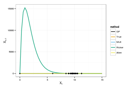
Phase-space diagram of the expected dynamics
true_means <- sapply(x_grid, f, 0, p)
mle_means <- sapply(x_grid, est$f, 0, est$p)
ricker_means <- sapply(x_grid, est$f, 0, ricker_bayes_pars[c(1,2)])
allen_means <- sapply(x_grid, f, 0, bayes_pars)

# myers_means <- sapply(x_grid, Myer_harvest, 0, myers_bayes_pars)

models <- data.frame(x=x_grid, GP=tgp_dat$y, True=true_means,
                     MLE=mle_means, Ricker = ricker_means,
                     Allen = allen_means)

models <- melt(models, id="x")
names(models) <- c("x", "method", "value")
plot_gp <- ggplot(tgp_dat) + geom_ribbon(aes(x,y,ymin=ymin,ymax=ymax), fill="gray80") +
    geom_line(data=models, aes(x, value, col=method), lwd=1, alpha=0.8) +
    geom_point(data=obs, aes(x,y), alpha=0.8) +
    xlab(expression(X[t])) + ylab(expression(X[t+1])) +
    scale_colour_manual(values=cbPalette)
print(plot_gp)
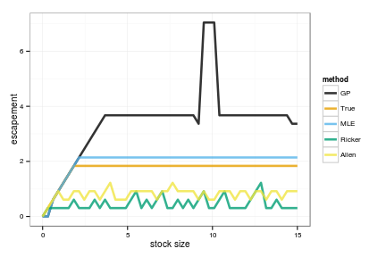
Optimal policies by value iteration
Compute the optimal policy under each model using stochastic dynamic programming. We begin with the policy based on the GP model,
MaxT = 1000
# uses expected values from GP, instead of integrating over posterior
#matrices_gp <- gp_transition_matrix(gp_dat$E_Ef, gp_dat$E_Vf, x_grid, h_grid)

# Integrate over posteriors
matrices_gp <- gp_transition_matrix(gp_dat$Ef_posterior, gp_dat$Vf_posterior, x_grid, h_grid)

# Solve the SDP using the GP-derived transition matrix
opt_gp <- value_iteration(matrices_gp, x_grid, h_grid, MaxT, xT, profit, delta, reward)
Determine the optimal policy based on the true and MLE models
matrices_true <- f_transition_matrix(f, p, x_grid, h_grid, sigma_g)
opt_true <- value_iteration(matrices_true, x_grid, h_grid, OptTime=MaxT, xT, profit, delta=delta)

matrices_estimated <- f_transition_matrix(est$f, est$p, x_grid, h_grid, est$sigma_g)
opt_estimated <- value_iteration(matrices_estimated, x_grid, h_grid, OptTime=MaxT, xT, profit, delta=delta)
Determine the optimal policy based on parametric Bayesian model
allen_f <- function(x,h,p) unname(f(x,h,p[c(2, 1, 3)]))
matrices_par_bayes <- parameter_uncertainty_SDP(allen_f, x_grid, h_grid, pardist, 4)
opt_par_bayes <- value_iteration(matrices_par_bayes, x_grid, h_grid, OptTime=MaxT, xT, profit, delta=delta)
Bayesian Ricker
ricker_f <- function(x, h, p) est$f(x, h, unname(p[c(2, 1)]))
matrices_alt <- parameter_uncertainty_SDP(ricker_f, x_grid, h_grid, as.matrix(ricker_pardist), 3)
opt_alt <- value_iteration(matrices_alt, x_grid, h_grid, OptTime=MaxT, xT, profit, delta=delta)
Assemble the data
OPT = data.frame(GP = opt_gp$D, True = opt_true$D, MLE = opt_estimated$D, Ricker = opt_alt$D, Allen = opt_par_bayes$D)
colorkey=cbPalette
names(colorkey) = names(OPT)
Graph of the optimal policies
policies <- melt(data.frame(stock=x_grid, sapply(OPT, function(x) x_grid[x])), id="stock")
names(policies) <- c("stock", "method", "value")

ggplot(policies, aes(stock, stock - value, color=method)) +
  geom_line(lwd=1.2, alpha=0.8) + xlab("stock size") + ylab("escapement")  +
  scale_colour_manual(values=colorkey)
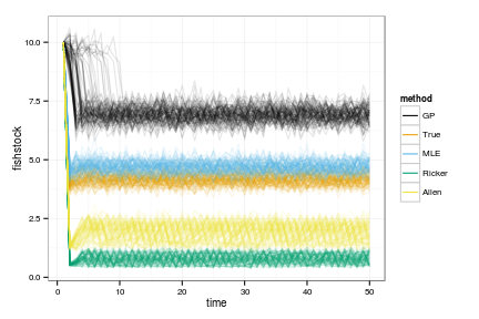
Simulate 100 realizations managed under each of the policies
sims <- lapply(OPT, function(D){
  set.seed(1)
  lapply(1:100, function(i)
    ForwardSimulate(f, p, x_grid, h_grid, x0, D, z_g, profit=profit, OptTime=OptTime)
  )
})

dat <- melt(sims, id=names(sims[[1]][[1]]))
dt <- data.table(dat)
setnames(dt, c("L1", "L2"), c("method", "reps"))
# Legend in original ordering please, not alphabetical:
dt$method = factor(dt$method, ordered=TRUE, levels=names(OPT))
ggplot(dt) +
  geom_line(aes(time, fishstock, group=interaction(reps,method), color=method), alpha=.1) +
  scale_colour_manual(values=colorkey, guide = guide_legend(override.aes = list(alpha = 1)))
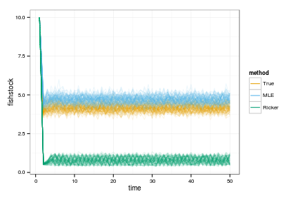
ggplot(dt[method %in% c("True", "Ricker", "MLE")]) +
  geom_line(aes(time, fishstock, group=interaction(reps,method), color=method), alpha=.1) +
  scale_colour_manual(values=colorkey, guide = guide_legend(override.aes = list(alpha = 1)))
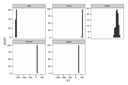
Profit <- dt[, sum(profit), by=c("reps", "method")]
Profit[, mean(V1), by="method"]
   method      V1
1:     GP -329.48
2:   True  109.25
3:    MLE   48.82
4: Ricker   23.09
5:  Allen   54.30
ggplot(Profit, aes(V1)) + geom_histogram() +
  facet_wrap(~method, scales = "free_y") + guides(legend.position = "none")
cboettig/nonparametric-bayes documentation built on May 13, 2019, 2:09 p.m.
R Package Documentation
Browse R Packages
We want your feedback!
Note that we can't provide technical support on individual packages. You should contact the package authors for that.
Comparison of Nonparametric Bayesian Gaussian Process estimates to standard the Parametric Bayesian approach
setwd("~/Documents/code/nonparametric-bayes/inst/examples/BUGS/")
Plotting and knitr options, (can generally be ignored)
library(knitcitations)
## Loading required package: bibtex
opts_chunk$set(tidy = FALSE, warning = FALSE, message = FALSE, cache = FALSE,
comment = NA, fig.width = 6, fig.height = 4)
library(ggplot2) # plotting
opts_knit$set(upload.fun = socialR::flickr.url)
theme_set(theme_bw(base_size = 10))
theme_update(panel.background = element_rect(fill = "transparent", colour = NA),
plot.background = element_rect(fill = "transparent", colour = NA))
cbPalette <- c("#000000", "#E69F00", "#56B4E9", "#009E73", "#F0E442", "#0072B2",
"#D55E00", "#CC79A7")
Load necessary libraries,
library(nonparametricbayes) # loads the rest as dependencies
Model and parameters
Uses the model derived in citet("10.1080/10236190412331335373"), of a Ricker-like growth curve with an allee effect, defined in the pdgControl package,
f <- Ricker
p <- c(1, 10)
K <- p[2]
C <- 5 # policy threshold
Various parameters defining noise dynamics, grid, and policy costs.
sigma_g <- 0.05
sigma_m <- 0.0
z_g <- function() rlnorm(1, 0, sigma_g)
z_m <- function() 1+(2*runif(1, 0, 1)-1) * sigma_m
x_grid <- seq(0, 1.5 * K, length=50)
h_grid <- x_grid
profit <- function(x,h) pmin(x, h) - 10*(x > C) # big penalty for violating threshold
delta <- 0.01
OptTime <- 50 # stationarity with unstable models is tricky thing
reward <- 0
xT <- 0
Xo <- K # observations start from
x0 <- Xo # simulation under policy starts from
Tobs <- 40
Sample Data
set.seed(1234)
#harvest <- sort(rep(seq(0, .5, length=7), 5))
x <- numeric(Tobs)
x[1] <- 6
nz <- 1
for(t in 1:(Tobs-1))
x[t+1] = z_g() * f(x[t], h=0, p=p)
obs <- data.frame(x = c(rep(0,nz),
pmax(rep(0,Tobs-1), x[1:(Tobs-1)])),
y = c(rep(0,nz),
x[2:Tobs]))
# plot(x)
Maximum Likelihood
est <- par_est(obs, init = c(r = p[1],
K = mean(obs$x[obs$x>0]),
s = sigma_g))
Non-parametric Bayes
#inv gamma has mean b / (a - 1) (assuming a>1) and variance b ^ 2 / ((a - 2) * (a - 1) ^ 2) (assuming a>2)
s2.p <- c(5,5)
d.p = c(10, 1/0.1)
Estimate the Gaussian Process (nonparametric Bayesian fit)
gp <- gp_mcmc(obs$x, y=obs$y, n=1e5, s2.p = s2.p, d.p = d.p)
gp_dat <- gp_predict(gp, x_grid, burnin=1e4, thin=300)
Show traces and posteriors against priors
plots <- summary_gp_mcmc(gp)
# Summarize the GP model
tgp_dat <-
data.frame( x = x_grid,
y = gp_dat$E_Ef,
ymin = gp_dat$E_Ef - 2 * sqrt(gp_dat$E_Vf),
ymax = gp_dat$E_Ef + 2 * sqrt(gp_dat$E_Vf) )
Parametric Bayes
We initiate the MCMC chain (init_p) using the true values of the parameters p from the simulation. While impossible in real data, this gives the parametric Bayesian approach the best chance at succeeding. y is the timeseries (recall obs has the $x_t$, $x_{t+1}$ pairs)
# a bit unfair to start with the correct values, but anyhow...
init_p = p
names(init_p) = c("r0", "K", "theta")
Error: 'names' attribute [3] must be the same length as the vector [2]
y <- obs$x[-1]
N=length(y);
We'll be using the JAGS Gibbs sampler, a recent open source BUGS implementation with an R interface that works on most platforms. We initialize the usual MCMC parameters; see ?jags for details.
jags.data <- list("N","y")
n.chains = 1
n.iter = 40000
n.burnin = floor(10000)
n.thin = max(1, floor(n.chains * (n.iter - n.burnin)/1000))
The actual model is defined in a model.file that contains an R function that is automatically translated into BUGS code by R2WinBUGS. The file defines the priors and the model, as seen when read in here
cat(readLines(con="bugmodel-UPrior.txt"), sep="\n")
model{
K ~ dunif(0.01, 40.0)
logr0 ~ dunif(-6.0, 6.0)
logtheta ~ dunif(-6.0, 6.0)
stdQ ~ dunif(0.0001,100)
stdR ~ dunif(0.0001,100)
# JAGS notation, mean, and precision ( reciprical of the variance, 1/sigma^2)
iQ <- 1/(stdQ*stdQ);
iR <- 1/(stdR*stdR);
r0 <- exp(logr0)
theta <- exp(logtheta)
x[1] ~ dunif(0,10)
for(t in 1:(N-1)){
mu[t] <- x[t] * exp(r0 * (1 - x[t]/K)* (x[t] - theta) / K )
x[t+1] ~ dnorm(mu[t],iQ)
}
for(t in 1:(N)){
y[t] ~ dnorm(x[t],iR)
}
}
We define which parameters to keep track of, and set the initial values of parameters in the transformed space used by the MCMC. We use logarithms to maintain strictly positive values of parameters where appropriate.
# Uniform priors on standard deviation terms
jags.params=c("K","logr0","logtheta","stdQ", "stdR")
jags.inits <- function(){
list("K"=init_p["K"],"logr0"=log(init_p["r0"]),"logtheta"=log(init_p["theta"]), "stdQ"=sqrt(0.05),"stdR"=sqrt(0.1),"x"=y,.RNG.name="base::Wichmann-Hill", .RNG.seed=123)
}
set.seed(12345)
time_jags <- system.time(
jagsfit <- jags(data=jags.data, inits=jags.inits, jags.params, n.chains=n.chains,
n.iter=n.iter, n.thin=n.thin, n.burnin=n.burnin,model.file="bugmodel-UPrior.txt")
)
Compiling model graph
Resolving undeclared variables
Allocating nodes
Graph Size: 365
Initializing model
time_jags <- unname(time_jags["elapsed"]);
Convergence diagnostics for parametric bayes
jags_matrix <- as.data.frame(as.mcmc.bugs(jagsfit$BUGSoutput))
par_posteriors <- melt(cbind(index = 1:dim(jags_matrix)[1], jags_matrix), id = "index")
# Traces
ggplot(par_posteriors) + geom_line(aes(index, value)) + facet_wrap(~ variable, scale="free", ncol=1)
## priors (untransformed variables)
K_prior <- function(x) dunif(x, 0.01, 40)
logr_prior <- function(x) dunif(x, -6, 6)
logtheta_prior <- function(x) dunif(x, -6, 6)
stdQ_prior <- function(x) dunif(x, 0.001, 100)
stdR_prior <- function(x) dunif(x, 0.001, 100)
par_priors <- list(K = K_prior, deviance = function(x) 0 * x,
logr0 = logr_prior, logtheta = logtheta_prior,
stdQ = stdQ_prior, stdR = stdR_prior)
par_prior_curves <- ddply(par_posteriors, "variable", function(dd){
grid <- seq(min(dd$value), max(dd$value), length = 100)
data.frame(value = grid, density = par_priors[[dd$variable[1]]](grid))
})
# posterior distributions
ggplot(par_posteriors, aes(value)) +
stat_density(geom="path", position="identity", alpha=0.7) +
geom_line(data=par_prior_curves, aes(x=value, y=density), col="red") +
facet_wrap(~ variable, scale="free", ncol=2)
# um, cleaner if we were just be using the long form, par_posterior
mcmc <- as.mcmc(jagsfit)
mcmcall <- mcmc[,-2]
who <- colnames(mcmcall)
who
[1] "K" "logr0" "logtheta" "stdQ" "stdR"
mcmcall <- cbind(mcmcall[,1],mcmcall[,2],mcmcall[,3],mcmcall[,4],mcmcall[,5])
colnames(mcmcall) <- who
pardist <- mcmcall
pardist[,2] = exp(pardist[,2]) # transform model parameters back first
pardist[,3] = exp(pardist[,3])
bayes_coef <- apply(pardist,2,mean)
bayes_pars <- unname(c(bayes_coef[2], bayes_coef[1], bayes_coef[3]))
bayes_pars
[1] 1.270 9.818 0.314
par_bayes_means <- sapply(x_grid, f, 0, bayes_pars)
Parametric Bayes based on the structurally wrong model
We initiate the MCMC chain (init_p) using the true values of the parameters p from the simulation. While impossible in real data, this gives the parametric Bayesian approach the best chance at succeeding. y is the timeseries (recall obs has the $x_t$, $x_{t+1}$ pairs)
init_p = p
names(init_p) = c("r0", "K")
y <- obs$x[-1]
N=length(y);
We'll be using the JAGS Gibbs sampler, a recent open source BUGS implementation with an R interface that works on most platforms. We initialize the usual MCMC parameters; see ?jags for details.
jags.data <- list("N","y")
n.chains = 1
n.iter = 40000
n.burnin = floor(10000)
n.thin = max(1, floor(n.chains * (n.iter - n.burnin)/1000))
The actual model is defined in a model.file that contains an R function that is automatically translated into BUGS code by R2WinBUGS. The file defines the priors and the model, as seen when read in here
cat(readLines(con="ricker-UPrior.txt"), sep="\n")
model{
K ~ dunif(0.01, 40.0)
logr0 ~ dunif(-6.0, 6.0)
stdQ ~ dunif(0.0001,100)
stdR ~ dunif(0.0001,100)
# JAGS notation, mean, and precision ( reciprical of the variance, 1/sigma^2)
iQ <- 1/(stdQ*stdQ);
iR <- 1/(stdR*stdR);
r0 <- exp(logr0)
x[1] ~ dunif(0,10)
for(t in 1:(N-1)){
mu[t] <- x[t] * exp(r0 * (1 - x[t]/K) / K )
x[t+1] ~ dnorm(mu[t],iQ)
}
for(t in 1:(N)){
y[t] ~ dnorm(x[t],iR)
}
}
We define which parameters to keep track of, and set the initial values of parameters in the transformed space used by the MCMC. We use logarithms to maintain strictly positive values of parameters where appropriate.
# Uniform priors on standard deviation terms
jags.params=c("K","logr0", "stdQ", "stdR")
jags.inits <- function(){
list("K"=init_p["K"],"logr0"=log(init_p["r0"]), "stdQ"=sqrt(0.05),"stdR"=sqrt(0.1),"x"=y,.RNG.name="base::Wichmann-Hill", .RNG.seed=123)
}
set.seed(12345)
time_jags <- system.time(
jagsfit <- jags(data=jags.data, inits=jags.inits, jags.params, n.chains=n.chains,
n.iter=n.iter, n.thin=n.thin, n.burnin=n.burnin,model.file="ricker-UPrior.txt")
)
Compiling model graph
Resolving undeclared variables
Allocating nodes
Graph Size: 325
Initializing model
time_jags <- unname(time_jags["elapsed"]);
Convergence diagnostics for parametric bayes Ricker model
jags_matrix <- as.data.frame(as.mcmc.bugs(jagsfit$BUGSoutput))
par_posteriors <- melt(cbind(index = 1:dim(jags_matrix)[1], jags_matrix), id = "index")
# Traces
ggplot(par_posteriors) + geom_line(aes(index, value)) +
facet_wrap(~ variable, scale="free", ncol=1)
## priors (untransformed variables)
K_prior <- function(x) dunif(x, 0.01, 40)
logr_prior <- function(x) dunif(x, -6, 6)
stdQ_prior <- function(x) dunif(x, 0.001, 100)
stdR_prior <- function(x) dunif(x, 0.001, 100)
par_priors <- list(K = K_prior, deviance = function(x) 0 * x, logr0 = logr_prior, stdQ = stdQ_prior, stdR = stdR_prior)
par_prior_curves <- ddply(par_posteriors, "variable", function(dd){
grid <- seq(min(dd$value), max(dd$value), length = 100)
data.frame(value = grid, density = par_priors[[dd$variable[1]]](grid))
})
# posterior distributions
ggplot(par_posteriors, aes(value)) +
stat_density(geom="path", position="identity", alpha=0.7) +
geom_line(data=par_prior_curves, aes(x=value, y=density), col="red") +
facet_wrap(~ variable, scale="free", ncol=2)
ricker_pardist <- jags_matrix[! names(jags_matrix) == "deviance" ]
ricker_pardist[,"logr0"] = exp(ricker_pardist[,"logr0"]) # transform model parameters back first
posterior.mode <- function(x) {
ux <- unique(x)
ux[which.max(tabulate(match(x, ux)))]
}
apply(ricker_pardist,2,mean)
K logr0 stdQ stdR
9.8075 9.0975 0.3128 0.3167
bayes_coef <- apply(ricker_pardist,2, posterior.mode) # much better estimates
ricker_bayes_pars <- unname(c(bayes_coef[2], bayes_coef[1]))
ricker_bayes_pars
[1] 10.73 9.73
Write the external bugs file
logr0_prior_p <- c(-6.0, 6.0)
logtheta_prior_p <- c(-6.0, 6.0)
logK_prior_p <- c(-6.0, 6.0)
stdQ_prior_p <- c(0.0001, 100)
stdR_prior_p <- c(0.0001, 100)
bugs.model <-
paste(sprintf(
"model{
logr0 ~ dunif(%s, %s)
logtheta ~ dunif(%s, %s)
logK ~ dunif(%s, %s)
stdQ ~ dunif(%s, %s)
stdR ~ dunif(%s, %s)",
logr0_prior_p[1], logr0_prior_p[2],
logtheta_prior_p[1], logtheta_prior_p[2],
logK_prior_p[1], logK_prior_p[2],
stdQ_prior_p[1], stdQ_prior_p[2],
stdR_prior_p[1], stdR_prior_p[2]),
"
iQ <- 1 / (stdQ * stdQ);
iR <- 1 / (stdR * stdR);
r0 <- exp(logr0)
theta <- exp(logtheta)
K <- exp(logK)
x[1] ~ dunif(0, 10)
for(t in 1:(N-1)){
mu[t] <- r0 * pow(abs(x[t]), theta) / (1 + pow(abs(x[t]), theta) / K)
x[t+1] ~ dnorm(mu[t], iQ)
}
for(t in 1:(N)){
y[t] ~ dnorm(x[t], iR)
}
}")
writeLines(bugs.model, "myers.bugs")
## priors (untransformed variables)
logK_prior <- function(x) dunif(x, logK_prior_p[1], logK_prior_p[2])
logr_prior <- function(x) dunif(x, logr0_prior_p[1], logr0_prior_p[2])
logtheta_prior <- function(x) dunif(x, logtheta_prior_p[1], logtheta_prior_p[2])
stdQ_prior <- function(x) dunif(x, stdQ_prior_p[1], stdQ_prior_p[2])
stdR_prior <- function(x) dunif(x, stdR_prior_p[1], stdR_prior_p[2])
Phase-space diagram of the expected dynamics
true_means <- sapply(x_grid, f, 0, p)
mle_means <- sapply(x_grid, est$f, 0, est$p)
ricker_means <- sapply(x_grid, est$f, 0, ricker_bayes_pars[c(1,2)])
allen_means <- sapply(x_grid, f, 0, bayes_pars)
# myers_means <- sapply(x_grid, Myer_harvest, 0, myers_bayes_pars)
models <- data.frame(x=x_grid, GP=tgp_dat$y, True=true_means,
MLE=mle_means, Ricker = ricker_means,
Allen = allen_means)
models <- melt(models, id="x")
names(models) <- c("x", "method", "value")
plot_gp <- ggplot(tgp_dat) + geom_ribbon(aes(x,y,ymin=ymin,ymax=ymax), fill="gray80") +
geom_line(data=models, aes(x, value, col=method), lwd=1, alpha=0.8) +
geom_point(data=obs, aes(x,y), alpha=0.8) +
xlab(expression(X[t])) + ylab(expression(X[t+1])) +
scale_colour_manual(values=cbPalette)
print(plot_gp)
Optimal policies by value iteration
Compute the optimal policy under each model using stochastic dynamic programming. We begin with the policy based on the GP model,
MaxT = 1000
# uses expected values from GP, instead of integrating over posterior
#matrices_gp <- gp_transition_matrix(gp_dat$E_Ef, gp_dat$E_Vf, x_grid, h_grid)
# Integrate over posteriors
matrices_gp <- gp_transition_matrix(gp_dat$Ef_posterior, gp_dat$Vf_posterior, x_grid, h_grid)
# Solve the SDP using the GP-derived transition matrix
opt_gp <- value_iteration(matrices_gp, x_grid, h_grid, MaxT, xT, profit, delta, reward)
Determine the optimal policy based on the true and MLE models
matrices_true <- f_transition_matrix(f, p, x_grid, h_grid, sigma_g)
opt_true <- value_iteration(matrices_true, x_grid, h_grid, OptTime=MaxT, xT, profit, delta=delta)
matrices_estimated <- f_transition_matrix(est$f, est$p, x_grid, h_grid, est$sigma_g)
opt_estimated <- value_iteration(matrices_estimated, x_grid, h_grid, OptTime=MaxT, xT, profit, delta=delta)
Determine the optimal policy based on parametric Bayesian model
allen_f <- function(x,h,p) unname(f(x,h,p[c(2, 1, 3)]))
matrices_par_bayes <- parameter_uncertainty_SDP(allen_f, x_grid, h_grid, pardist, 4)
opt_par_bayes <- value_iteration(matrices_par_bayes, x_grid, h_grid, OptTime=MaxT, xT, profit, delta=delta)
Bayesian Ricker
ricker_f <- function(x, h, p) est$f(x, h, unname(p[c(2, 1)]))
matrices_alt <- parameter_uncertainty_SDP(ricker_f, x_grid, h_grid, as.matrix(ricker_pardist), 3)
opt_alt <- value_iteration(matrices_alt, x_grid, h_grid, OptTime=MaxT, xT, profit, delta=delta)
Assemble the data
OPT = data.frame(GP = opt_gp$D, True = opt_true$D, MLE = opt_estimated$D, Ricker = opt_alt$D, Allen = opt_par_bayes$D)
colorkey=cbPalette
names(colorkey) = names(OPT)
Graph of the optimal policies
policies <- melt(data.frame(stock=x_grid, sapply(OPT, function(x) x_grid[x])), id="stock")
names(policies) <- c("stock", "method", "value")
ggplot(policies, aes(stock, stock - value, color=method)) +
geom_line(lwd=1.2, alpha=0.8) + xlab("stock size") + ylab("escapement") +
scale_colour_manual(values=colorkey)
Simulate 100 realizations managed under each of the policies
sims <- lapply(OPT, function(D){
set.seed(1)
lapply(1:100, function(i)
ForwardSimulate(f, p, x_grid, h_grid, x0, D, z_g, profit=profit, OptTime=OptTime)
)
})
dat <- melt(sims, id=names(sims[[1]][[1]]))
dt <- data.table(dat)
setnames(dt, c("L1", "L2"), c("method", "reps"))
# Legend in original ordering please, not alphabetical:
dt$method = factor(dt$method, ordered=TRUE, levels=names(OPT))
ggplot(dt) +
geom_line(aes(time, fishstock, group=interaction(reps,method), color=method), alpha=.1) +
scale_colour_manual(values=colorkey, guide = guide_legend(override.aes = list(alpha = 1)))
ggplot(dt[method %in% c("True", "Ricker", "MLE")]) +
geom_line(aes(time, fishstock, group=interaction(reps,method), color=method), alpha=.1) +
scale_colour_manual(values=colorkey, guide = guide_legend(override.aes = list(alpha = 1)))
Profit <- dt[, sum(profit), by=c("reps", "method")]
Profit[, mean(V1), by="method"]
method V1
1: GP -329.48
2: True 109.25
3: MLE 48.82
4: Ricker 23.09
5: Allen 54.30
ggplot(Profit, aes(V1)) + geom_histogram() +
facet_wrap(~method, scales = "free_y") + guides(legend.position = "none")
R Package Documentation
Browse R Packages
We want your feedback!
Note that we can't provide technical support on individual packages. You should contact the package authors for that.
Embedding an R snippet on your website
Add the following code to your website.
For more information on customizing the embed code, read Embedding Snippets.