inst/examples/admb-example.md

In cboettig/nonparametric-bayes: Nonparametric Bayes inference for ecological models

Learning ADMB

Plotting and knitr options, (can generally be ignored)

Model and parameters

f <- function(x,h,p)  x * exp(p[1] * (1 - x / p[2]) * (x - p[3]) / p[2] ) 
p <- c(1, 10, 5)
K <- 10  # approx, a li'l' less
Xo <- 6 # approx, a li'l' less

Various parameters defining noise dynamics, grid, and policy costs.

sigma_g <- 0.1
z_g <- function() rlnorm(1,0, sigma_g)
x_grid <- seq(0, 1.5 * K, length=50)
Tobs <- 40
set.seed(123)

Sample Data

x <- numeric(Tobs)
x[1] <- Xo
for(t in 1:(Tobs-1))
  x[t+1] = z_g() * f(x[t], h=0, p=p)
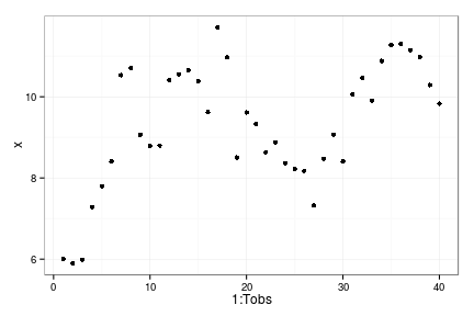
qplot(1:Tobs, x)

Maximum Likelihood "by hand"

STABLIZE = 1e-10
n = length(x)
mloglik <- function(pars){ 
  r = pars[1]; k = pars[2]; c = pars[3]; s = pars[4];
  mu = (x+STABLIZE) * exp( r * (1 - x / (k+STABLIZE)) * (x - c) / (k + STABLIZE));
  mu = pmin(1e100, mu) # avoid infinite values 
  f = 0.5 * n * log(2 * pi) + n * log(s + STABLIZE) + 0.5 * sum(x - mu + STABLIZE)^2/ (s + STABLIZE)^2;

  f
  }

Starting from the true values we mostly just shrink the noise parameter:

init <- c(p, sigma_g)
mloglik(init) #true minus loglik

[1] -35.72

o <- optim(init, mloglik, method="L", lower=1e-5, upper=1e5)
o$value

[1] -247.6

o$par

[1] 0.9967297 9.9813554 5.1742699 0.0008183

While starting from arbitrary values we still find the optim.

init <- c(1,1,1,1)  
init <- c(p, sigma_g)
mloglik(init) #true minus loglik

[1] -35.72

o <- optim(init, mloglik, method="L", lower=1e-5, upper=1e5)
o$value

[1] -247.6

o$par

[1] 0.9967297 9.9813554 5.1742699 0.0008183

Okay, now lets try admb. We use R2admb which is just a convenient way to write our data and parameters into an admb file.

# install_github("R2admb", "bbolker", subdir="R2admb") # dev version
library(R2admb)

ADMB definition

We still need to define the model using ADMB notation in the procedure section. This is mostly like R or C++, with the exception of special functions like square in place of ^2, norm2 for the sum of squares, and elem_prod istead of * for the element-wise product of two arrays. The constant pi is given as M_PI, as typical of C/C++ libraries. Where these other functions are defined I'm not sure, but some useful guides to ADMB vector/matrix operations or an (undefined) list of keywords...

The equivalent model

model <- 
paste("
PARAMETER_SECTION
  vector mu(1,n) // per capita mort prob

PROCEDURE_SECTION
  mu = log(x) + r * elem_prod((1 - x / k), (x - c) / k);
  f = 0.5 * n * log(2 * M_PI) + n * log(s) + 0.5 * norm2(x - exp(mu)) / square(s);
")
writeLines(model, "model.tpl")

Without explicit handling of the overflow errors, ADMB does not give us reliable estimates with arbitrary starting conditions

setup_admb("/var/admb")

[1] "/var/admb"

df <- data.frame(x=x)
params <- list(r = 1, k = 1, c = 1, s = 1) ## starting parameters
bounds <- list(r = c(1e-10, 1e3), k=c(1e-10, 1e3), c=c(1e-10, 1e3), s = c(1e-5,1e3)) ## bounds
dat <- c(list(n = nrow(df)), df)
m1 <- do_admb("model",
              data = dat,
              params = params,
              bounds = bounds,
              run.opts = run.control(checkparam="write",
                                     checkdata="write", clean=FALSE))
m1

Model file: model_gen 
Negative log-likelihood: 146.5 
Coefficients:
     r      k      c      s 
0.9992 1.0023 1.0004 9.4369 

But does fine with good starting values. Hmm.. thought that was supposed to be the other way around...

params <- list(r = 1, k = 10, c = 5, s = .1) ## starting parameters

m1 <- do_admb("model",
              data = dat,
              params = params,
              bounds = bounds,
              run.opts = run.control(checkparam="write",
                                     checkdata="write"))

Warning: running command './model_gen > model_gen.out' had status 1

m1

Model file: model_gen 
Negative log-likelihood: -423.8 
Coefficients:
        r         k         c         s 
2.025e-10 9.498e+00 1.051e+01 1.000e-05 

Which finds a better optim (though substantailly overfit in reality)

Hans suggests adding an error term in the function definitions rather than in limiting the bounds or log transforming the variables:

The most common plase where this goes wrong is 1/0, log(0), sqrt(0), pow(0,1) etc. Your suggestion is OK, but usually I prefer to put in log(1e-10+my_expression), sqrt(1e-10+my_expression), pow(1e-10+my_expression,1)

cboettig/nonparametric-bayes documentation built on May 13, 2019, 2:09 p.m.