inst/examples/may79-example.md

In cboettig/nonparametric-bayes: Nonparametric Bayes inference for ecological models

GP Example using the May (1979) bistable model

## Loading required package: bibtex

## Warning: replacing previous import 'write.bib' when loading 'pkgmaker'

f <- May
p <- c(r = .75, k = 10, a=1.3, H=1, Q = 3)
K <- 8 

We use the model of May et. al. (1979).

sigma_g <- 0.04
z_g <- function(sigma_g) rlnorm(1, 0, sigma_g) #1+(2*runif(1, 0,  1)-1)*sigma_g #
x_grid <- seq(0, 1.5 * K, length=101)
h_grid <- x_grid
profit = function(x,h) pmin(x, h)
delta <- 0.01
OptTime = 20
reward = profit(x_grid[length(x_grid)], x_grid[length(x_grid)]) + 1 / (1 - delta) ^ OptTime 

With parameters 0.75, 10, 1.3, 1, 3.

xT <- x_grid[2]
x_0_observed <- x_grid[60]

Tobs <- 100
x <- numeric(Tobs)
x[1] <- x_0_observed
for(t in 1:(Tobs-1))
  x[t+1] = z_g(sigma_g) * f(x[t], h=0, p=p)
plot(x)

We simulate data under this model, starting from a size of 7.08.

obs <- data.frame(x=c(0,x[1:(Tobs-1)]),y=c(0,x[2:Tobs]))

We consider the observations as ordered pairs of observations of current stock size $x_t$ and observed stock in the following year, $x_{t+1}$. We add the pseudo-observation of $0,0$. Alternatively we could condition strictly on solutions passing through the origin, though in practice the weaker assumption is often sufficient.

estf <- function(p){
  mu <- log(obs$x) + p["r"]*(1-obs$x/p["K"])
  -sum(dlnorm(obs$y, mu, p["s"]), log=TRUE)
}
o <- optim(par = c(r=1,K=mean(x),s=1), estf, method="L", lower=c(1e-3,1e-3,1e-3))
f_alt <- Ricker
p_alt <- c(o$par['r'], o$par['K'])
sigma_g_alt <- o$par['s']

gp <- bgp(X=obs$x, XX=x_grid, Z=obs$y, verb=0,
          meanfn="linear", bprior="b0", BTE=c(2000,6000,2), m0r1=FALSE, 
          corr="exp", trace=TRUE, beta = c(0,0),
          s2.p = c(50,50), d.p = c(10, 1/0.01, 10, 1/0.01), nug.p = c(10, 1/0.01, 10, 1/0.01),
          s2.lam = "fixed", d.lam = "fixed", nug.lam = "fixed", 
          tau2.lam = "fixed", tau2.p = c(50,1))

We fit a Gaussian process with

V <- gp$ZZ.ks2
Ef = gp$ZZ.km
tgp_dat <- data.frame(x   = gp$XX[[1]], 
                  y   = gp$ZZ.km, 
                 ymin = gp$ZZ.km - 1.96 * sqrt(gp$ZZ.ks2), 
                 ymax = gp$ZZ.km + 1.96 * sqrt(gp$ZZ.ks2))

true <- data.frame(x=x_grid, y=sapply(x_grid,f, 0, p))
ggplot(tgp_dat)  + geom_ribbon(aes(x,y,ymin=ymin,ymax=ymax), fill="gray80") +
  geom_line(aes(x,y)) + geom_point(data=obs, aes(x,y)) +
  geom_line(data=true, aes(x,y), col='red', lty=2)

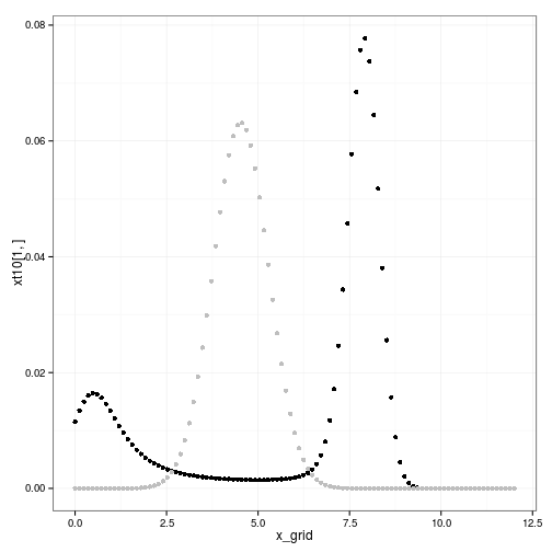
The transition matrix of the inferred process

X <- numeric(length(x_grid))
X[38] = 1
h <- 0

F_ <- gp_F(h, Ef, V, x_grid)
xt1 <- X %*% F_
xt10 <- xt1
for(s in 1:OptTime)
  xt10 <- xt10 %*% F_
qplot(x_grid, xt10[1,]) + geom_point(aes(y=xt1[1,]), col="grey")

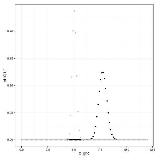
F_true <- par_F(h, f, p, x_grid, sigma_g)
yt1 <- X %*% F_true
yt10 <- yt1
for(s in 1:OptTime)
  yt10 <- yt10 %*% F_true
qplot(x_grid, yt10[1,]) + geom_point(aes(y=yt1[1,]), col="grey")

transition <- melt(data.frame(x = x_grid, gp = xt1[1,], parametric = yt1[1,]), id="x")
ggplot(transition) + geom_point(aes(x,value, col=variable))

matrices_gp <- gp_transition_matrix(Ef, V, x_grid, h_grid)
opt_gp <- find_dp_optim(matrices_gp, x_grid, h_grid, OptTime, xT, profit, delta, reward=reward)

matrices_true <- f_transition_matrix(f, p, x_grid, h_grid, sigma_g)
opt_true <- find_dp_optim(matrices_true, x_grid, h_grid, OptTime, xT, profit, delta=delta, reward = reward)

matrices_estimated <- f_transition_matrix(f_alt, p_alt, x_grid, h_grid, sigma_g_alt)
opt_estimated <- find_dp_optim(matrices_estimated, x_grid, h_grid, OptTime, xT, profit, delta=delta, reward = reward)

policies <- melt(data.frame(stock=x_grid, 
                            GP = x_grid[opt_gp$D[,1]], 
                            Exact = x_grid[opt_true$D[,1]],
                            Approx = x_grid[opt_estimated$D[,1]]),
                  id="stock")

policy_plot <- ggplot(policies, aes(stock, stock - value, color=variable)) +
  geom_point() + xlab("stock size") + ylab("escapement") 
policy_plot

z_g <- function() rlnorm(1,0, sigma_g)

set.seed(1)
sim_gp <- ForwardSimulate(f, p, x_grid, h_grid, K, opt_gp$D, z_g, profit=profit)
set.seed(1)
sim_true <- ForwardSimulate(f, p, x_grid, h_grid, K, opt_true$D, z_g, profit=profit)
set.seed(1)
sim_est <- ForwardSimulate(f, p, x_grid, h_grid, K, opt_estimated$D, z_g, profit=profit)

dat <- list(est = sim_est, gp = sim_gp, true = sim_true)
dat <- melt(dat, id=names(dat[[1]]))
dt <- data.table(dat)
setnames(dt, "L1", "method") 

ggplot(dt) + geom_line(aes(time,fishstock, color=method))

ggplot(dt) + geom_line(aes(time,harvest, color=method))

c( gp = sum(sim_gp$profit), true = sum(sim_true$profit), est = sum(sim_est$profit))

    gp   true    est 
 8.469 19.680 10.200 

May RM, Beddington JR, Clark CW, Holt SJ and Laws RM (1979). “Management of Multispecies Fisheries.” Science, 205. ISSN 0036-8075, http://dx.doi.org/10.1126/science.205.4403.267.

cboettig/nonparametric-bayes documentation built on May 13, 2019, 2:09 p.m.