inst/examples/pomp-example.md

In cboettig/nonparametric-bayes: Nonparametric Bayes inference for ecological models

library(pomp)

## Loading required package: mvtnorm

## Loading required package: subplex

## Loading required package: deSolve

opts_knit$set(upload.fun = socialR::flickr.url)
options(flickr_tags = "nonparametric-bayes")

process.sim <- function(x, t, params, delta.t, ...) {
    # r = 0.75, K = 10, Q = 3, H = 1, a = 1.3
    r <- params["r"]
    K <- params["K"]
    Q <- params["Q"]
    H <- params["H"]
    a <- params["a"]
    sigma <- params["sigma"]
    X <- x["X"]
    epsilon <- exp(rlnorm(n = 1, mean = 0, sd = sigma))

    c(X = unname(X * exp(r * delta.t * (1 - X/K) - a * X^(Q - 1)/(X^Q + H^Q)) * 
        epsilon))
}

measure.sim <- function(x, t, params, ...) {
    tau <- params["tau"]
    X <- x["X"]
    y <- c(Y = unname(rlnorm(n = 1, meanlog = log(X), sd = tau)))
}

Create a container of class pomp

may <- pomp(data = data.frame(time = 1:100, Y = NA), times = "time", 
    rprocess = discrete.time.sim(step.fun = process.sim, delta.t = 1), rmeasure = measure.sim, 
    t0 = 0)

Parameters and an initial condition

theta <- c(r = 0.75, K = 10, Q = 3, H = 1, a = 1.3, sigma = 0.2, 
    tau = 0.1, X.0 = 5)

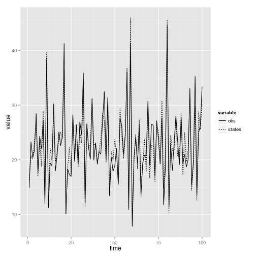
Simulate

dat <- simulate(may, params = theta, obs = TRUE, states = TRUE)
library(reshape2)
library(ggplot2)
dt <- melt(dat)[3:5]
names(dt) = c("time", "value", "variable")
ggplot(dt, aes(time, value, lty = variable)) + geom_line()

Note that simulate returns an instance of our object, with the data column filled in. This is not true if we give it arguments such as state or obs = TRUE as above. However, when we query for observed and true states in this way, the simulated data is not stored in our object. We must assign it with may <- pomp(data = ... where data is a data frame with columns "time" and "Y". This is much simpler if we use the default return:

may <- simulate(may, params = theta)

Measurement density

measure.density <- function(y, x, t, params, log, ...) {
    tau <- params["tau"]
    ## state at time t:
    X <- x["X"]
    ## observation at time t:
    Y <- y["Y"]
    ## compute the likelihood of Y|X,tau
    f <- dlnorm(x = Y, meanlog = log(X), sdlog = tau, log = log)

}

Add to our container

may <- pomp(may, dmeasure = measure.density)

Optionally, work in the transformed variable space instead by providing parameter and inverse parameter transforms.

may <- pomp(may, parameter.transform = function(params, ...) {
    exp(params)
}, parameter.inv.transform = function(params, ...) {
    log(params)
})

Run the particle filter. Note that this evaluates the likelihood of our simulated data (stored in the object) at the given (true) parameters.

pf <- pfilter(may, params = theta, Np = 1000)
logLik(pf)

## [1] -304.7

Here we go, estimate the model by particle filter. This'll be slow...

theta.guess <- theta + c(abs(rnorm(length(theta)-1)),0)
estpars <- names(theta[1:7]) # which pars should be estimated. lets try and get them all
rw.sd <- theta[1:7]/(50*theta[1:7]) # a named vector of random walk values. This sets it to 0.02 for all pars
system.time(mf <- 
  mif(may, Nmif = 10, # Number of iterations
      start = theta.guess, # Starting value of parameters
      transform = TRUE, # work in transformed parameter space (e.g. logs avoid neg par values)
      pars = estpars,  # which parameters to estimate (others fixed at starting value)
      rw.sd = rw.sd, # random walk width
      Np = 200, # Number of particles
      var.factor = 4, # scaling factor for random walk sd
      ic.lag = 10, # fixed lag
      cooling.factor = 0.999, # exponential cooling
      max.fail = 10) # internal tolerance
)

##    user  system elapsed 
##  22.018   0.008  22.106

compare.mif(mf)

coef(mf)

##       r       K       Q       H       a   sigma     tau     X.0 
##  0.6985 10.2655  4.0470  1.2844  1.6782  0.1587  0.1711  5.0000

logLik(mf)

## [1] -314.4

pf_est <- pfilter(may, params = theta.guess, Np = 1000)
logLik(pf_est)  # initial loglik

## [1] -441.9

These functions apply to replicated mifs above.

theta.true <- coef(may)
theta.mif <- apply(sapply(mf, coef), 1, mean)

## Error: no method for coercing this S4 class to a vector

loglik.mif <- replicate(n = 10, logLik(pfilter(mf[[1]], params = theta.mif, 
    Np = 10000)))

## recover called non-interactively; frames dumped, use debugger() to view
## recover called non-interactively; frames dumped, use debugger() to view

## Error: error in evaluating the argument 'object' in selecting a method for
## function 'logLik': Error in pfilter(mf[[1]], params = theta.mif, Np =
## 10000) : error in evaluating the argument 'object' in selecting a method
## for function 'pfilter': Error in mf[[1]] : this S4 class is not
## subsettable

bl <- mean(loglik.mif)

## Error: object 'loglik.mif' not found

loglik.mif.est <- bl + log(mean(exp(loglik.mif - bl)))

## Error: object 'bl' not found

loglik.mif.se <- sd(exp(loglik.mif - bl))/exp(loglik.mif.est - bl)

## Error: object 'loglik.mif' not found

cboettig/nonparametric-bayes documentation built on May 13, 2019, 2:09 p.m.