inst/examples/semi-analytic-posteriors.md

In cboettig/nonparametric-bayes: Nonparametric Bayes inference for ecological models

Semi-analytic posteriors

Generating Model and parameters

Ricker model, parameterized as

$$X_{t+1} = X_t r e^{-\beta X_t + \sigma Z_t}$$

for random unit normal $Z_t$

f <- function(x,h,p)  x * p[1] * exp(-x * p[2]) 
p <- c(exp(1), 1/10)
K <- 10  # approx, a li'l' less
Xo <- 1 # approx, a li'l' less

sigma_g <- 0.1
z_g <- function() rlnorm(1,0, sigma_g)
x_grid <- seq(0, 1.5 * K, length=50)
N <- 40
set.seed(123)

Sample Data

x <- numeric(N)
x[1] <- Xo
for(t in 1:(N-1))
  x[t+1] = z_g() * f(x[t], h=0, p=p)
qplot(1:N, x)

Compute the posterior after marginalizing over $r$ and $\sigma$ parameters:

$$P(\beta | X) $$

Mt <- function(t, beta) log(x[t+1]) - log(x[t]) + beta * x[t]
beta_grid = seq(1e-5, 2, by=1e-3)

P_B.X <- sapply(beta_grid, function(beta){
  Mt_vec = sapply(1:(N-1), Mt, beta)
  sum_of_squares <- sum(Mt_vec^2)
  square_of_sums <- sum(Mt_vec)^2
  0.5 ^ (N/2-1) * (sum_of_squares - square_of_sums/(N-1)) ^ (N/2-1) / gamma(N/2-1)
  })

qplot(beta_grid, -log(P_B.X))

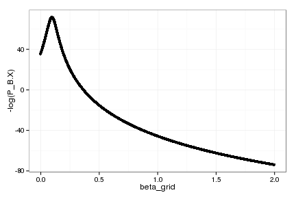
beta_grid[which.min(P_B.X)]

[1] 0.09801

Estimating the Allen model:

$$X_{t+1} = X_t \exp\left(r \left(1 - \frac{X_t}{K} \right\left(\frac{X - C}{K}\right)\right) $$

First re-parameterize so we can isolate an additive parameter, using standard quadratic form,

$$X_{t+1} = X_t \exp(c + b X_t + a X_t^2) $$

Where $c = \tfrac{-rC}{K}$, $b = \tfrac{r}{K}\left(\tfrac{C}{K} + 1\right)$, and $a = \tfrac{r}{K^2}$. Then after integrating out $c$ and $\sigma$ we have

Mt <- function(t, a, b)  log(x[t+1]) - log(x[t]) - b * x[t] + a * x[t] ^ 2

Choosing a sensible grid is a bit more tricky following the transformation, particularly $b$ can be negative or positive, and much larger in magnitude than any of the original parameters. $a$ on the other hand, can be reasonably restricted:

b_grid = seq(0, .1, length=100)
a_grid = seq(0, .1, length=100)

We define the probability as a function of the remaining two parameters,

prob <- function(a, b){
  Mt_vec = sapply(1:(N-1), Mt, a, b)
  sum_of_squares <- sum(Mt_vec^2)
  square_of_sums <- sum(Mt_vec)^2
0.5 ^ (N/2-1) * (sum_of_squares - square_of_sums/(N-1)) ^ (N/2-1) / gamma(N/2-1)
}

and loop over the grid on each

P_a_b.X <- sapply(a_grid, function(a)
                sapply(b_grid, function(b) prob(a, b)))

We summarize with a contour plot

  df = melt(P_a_b.X)
names(df) = c("a", "b", "lik")
ggplot(df, aes(a_grid[a], b_grid[b], z=-log(lik))) + 
  stat_contour(aes(color=..level..), binwidth=1) +
  coord_cartesian(ylim=c(0, .025), xlim=c(0,.05))

Estimating the Myers model on this data:

$$X_{t+1} = Z_t \frac{r X_t^{\theta}}{1 + X_t^{\theta} / K}$$

With $Z_t$ lognormal, unit mean, std $\sigma$.

Mt <- function(t, theta, K) log(x[t+1]) - theta * log(x[t]) + log(1 + x[t] ^ theta / K) 
theta_grid = seq(1e-5, 5, length=100)
K_grid = seq(1e-5, 30, length=100)

prob <- function(theta, K){
  Mt_vec = sapply(1:(N-1), Mt, theta, K)
  sum_of_squares <- sum(Mt_vec^2)
  square_of_sums <- sum(Mt_vec)^2
0.5 ^ (N/2-1) * (sum_of_squares - square_of_sums/(N-1)) ^ (N/2-1) / gamma(N/2-1)
}



P_theta_K.X <- sapply(theta_grid, function(theta)
                sapply(K_grid, function(k) prob(theta, k)))


require(reshape2)
df = melt(P_theta_K.X)
names(df) = c("theta", "K", "lik")
ggplot(df, aes(theta_grid[theta], K_grid[K], z=-log(lik))) + stat_contour(aes(color=..level..), binwidth=3)

cboettig/nonparametric-bayes documentation built on May 13, 2019, 2:09 p.m.