In fbertran/Patterns: Deciphering Biological Networks with Patterned Heterogeneous Measurements
knitr::opts_chunk$set(
  collapse = TRUE,
  comment = "#>",
  fig.path = "man/figures/README-",
  out.width = "100%",
  dpi=300,fig.width=7,
  fig.keep="all"
)
Patterns 
A modeling tool dedicated to biological network modeling to decipher Biological Networks with Patterned Heterogeneous (e.g. multiOmics) Measurements
Frédéric Bertrand and Myriam Maumy-Bertrand


It is designed to work with patterned data. Famous examples of problems related to patterned data are:
- recovering signals in networks after a stimulation (cascade network reverse engineering),
- analysing periodic signals.
It allows for single or joint modeling of, for instance, genes and proteins.
- It starts with the selection of the actors that will be the used in the reverse engineering upcoming step. An actor can be included in that selection based on its differential effects (for instance gene expression or protein abundance) or on its time course profile.
- Wrappers for actors clustering functions and cluster analysis are provided.
- It also allows reverse engineering of biological networks taking into account the observed time course patterns of the actors. Interactions between clusters of actors can be set by the user. Any number of clusters can be activated at a single time.
- Many inference functions are provided with the
Patterns package and dedicated to get specific features for the inferred network such as sparsity, robust links, high confidence links or stable through resampling links.
- lasso, from the
lars package
- lasso, from the
glmnet package. An unweighted and a weighted version of the algorithm are available
- spls, from the
spls package
- elasticnet, from the
elasticnet package
- stability selection, from the
c060 package implementation of stability selection
- weighted stability selection, a new weighted version of the
c060 package implementation of stability selection that I created for the package
- robust, lasso from the
lars package with light random Gaussian noise added to the explanatory variables
- selectboost, from the
selectboost package. The selectboost algorithm looks for the more stable links against resampling that takes into account the correlated structure of the predictors
- weighted selectboost, a new weighted version of the
selectboost.
- Some simulation and prediction tools are also available for cascade networks.
- Examples of use with microarray or RNA-Seq data are provided.
The weights are viewed as a penalty factors in the penalized regression model: it is a number that multiplies the lambda value in the minimization problem to allow differential shrinkage, Friedman et al. 2010, equation 1 page 3. If equal to 0, it implies no shrinkage, and that variable is always included in the model. Default is 1 for all variables. Infinity means that the variable is excluded from the model. Note that the weights are rescaled to sum to the number of variables.
A word for those that have been using our seminal work, the Cascade package that we created several years ago and that was a very efficient network reverse engineering tool for cascade networks
(Jung, N., Bertrand, F., Bahram, S., Vallat, L., and Maumy-Bertrand, M. (2014), https://doi.org/10.1093/bioinformatics/btt705, https://cran.r-project.org/package=Cascade, https://github.com/fbertran/Cascade and https://fbertran.github.io/Cascade/).
The Patterns package is more than (at least) a threeway major extension of the Cascade package :
- any number of groups can be used whereas in the
Cascade package only 1 group for each timepoint could be created, which prevented the users to create homogeneous clusters of genes in datasets that featured more than a few dozens of genes.
- custom $F$ matrices shapes whereas in the
Cascade package only 1 shape was provided:
- interaction between groups
- custom design of inner cells of the $F$ matrix
- the custom $F$ matrices allow to deal with heteregeneous networks with several kinds of actors such as mixing genes and proteins in a single network to perform joint inference.
- about nine inference algorithms are provided, whereas 1 (lasso) in
Cascade.
Hence the Patterns package should be viewed more as a completely new modelling tools than as an extension of the Cascade package.
This website and these examples were created by F. Bertrand and M. Maumy-Bertrand.
Installation
You can install the released version of Patterns from CRAN with:
install.packages("Patterns")
You can install the development version of Patterns from github with:
devtools::install_github("fbertran/Patterns")
Examples
Data management
Import Cascade Data (repeated measurements on several subjects) from the CascadeData package and turn them into a omics array object. The second line makes sure the CascadeData package is installed.
library(Patterns)
if(!require(CascadeData)){install.packages("CascadeData")}
data(micro_US)
micro_US<-as.omics_array(micro_US[1:100,],time=c(60,90,210,390),subject=6)
str(micro_US)
Get a summay and plots of the data:
summary(micro_US)
plot(micro_US)
Gene selection
There are several functions to carry out gene selection before the inference. They are detailed in the vignette of the package.
Data simulation
Let's simulate some cascade data and then do some reverse engineering.
We first design the F matrix for $T_i=4$ times and $Ngrp=4$ groups. The Fmatobject is an array of sizes $(T_i,T-i,Ngrp^2)=(4,4,16)$.
Ti<-4
Ngrp<-4

Fmat=array(0,dim=c(Ti,Ti,Ngrp^2))

for(i in 1:(Ti^2)){
  if(((i-1) %% Ti) > (i-1) %/% Ti){
    Fmat[,,i][outer(1:Ti,1:Ti,function(x,y){0<(x-y) & (x-y)<2})]<-1
    }
}
The Patterns function CascadeFinit is an utility function to easily define such an F matrix.
Fbis=Patterns::CascadeFinit(Ti,Ngrp,low.trig=FALSE)
str(Fbis)
Check if the two matrices Fmat and Fbis are identical.
print(all(Fmat==Fbis))
End of F matrix definition.
Fmat[,,3]<-Fmat[,,3]*0.2
Fmat[3,1,3]<-1
Fmat[4,2,3]<-1
Fmat[,,4]<-Fmat[,,3]*0.3
Fmat[4,1,4]<-1
Fmat[,,8]<-Fmat[,,3]
We set the seed to make the results reproducible and draw a scale free random network.
set.seed(1)
Net<-Patterns::network_random(
  nb=100,
  time_label=rep(1:4,each=25),
  exp=1,
  init=1,
  regul=round(rexp(100,1))+1,
  min_expr=0.1,
  max_expr=2,
  casc.level=0.4
)
Net@F<-Fmat
str(Net)
Plot the simulated network.
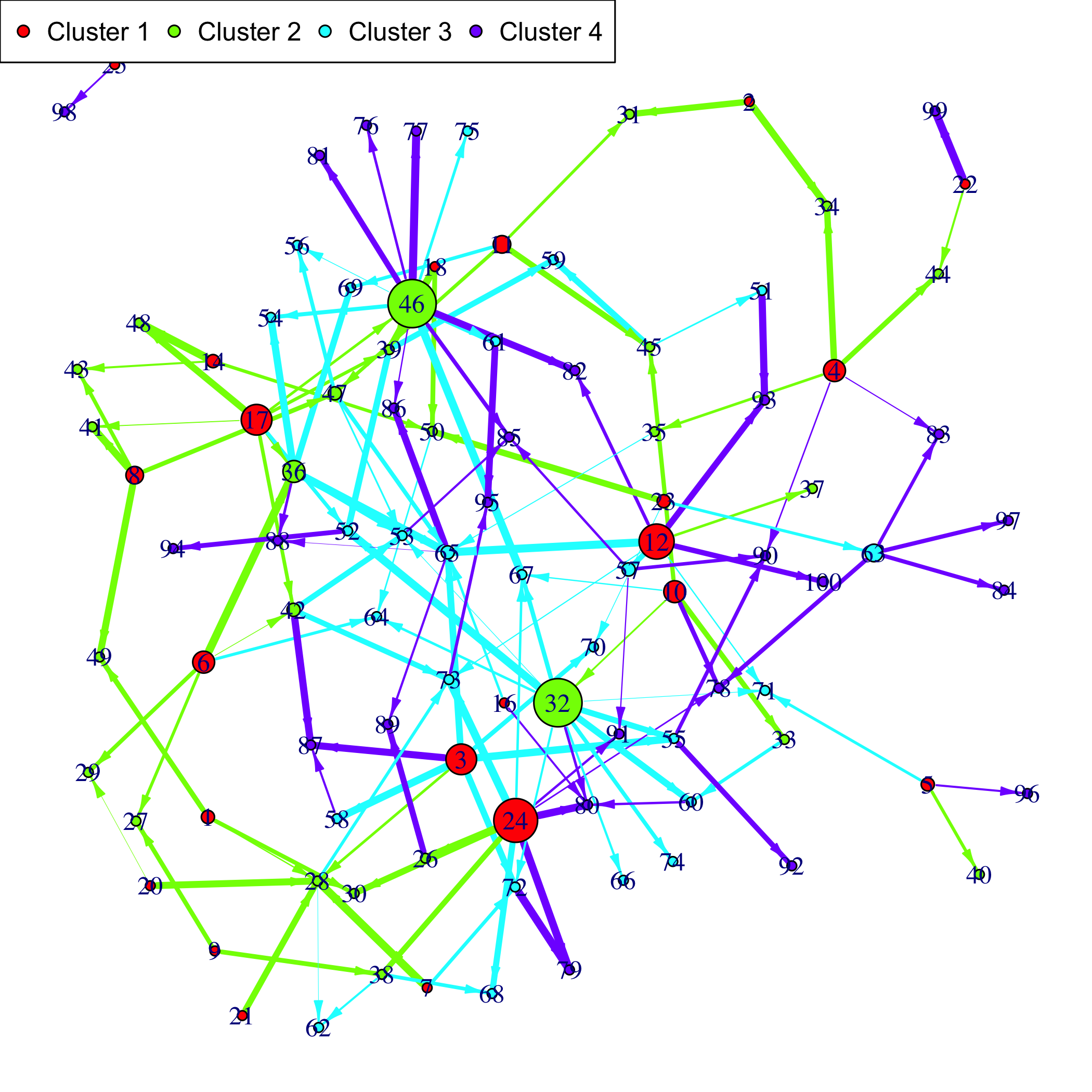
Patterns::plot(Net, choice="network")
If a gene clustering is known, it can be used as a coloring scheme.
plot(Net, choice="network", gr=rep(1:4,each=25))
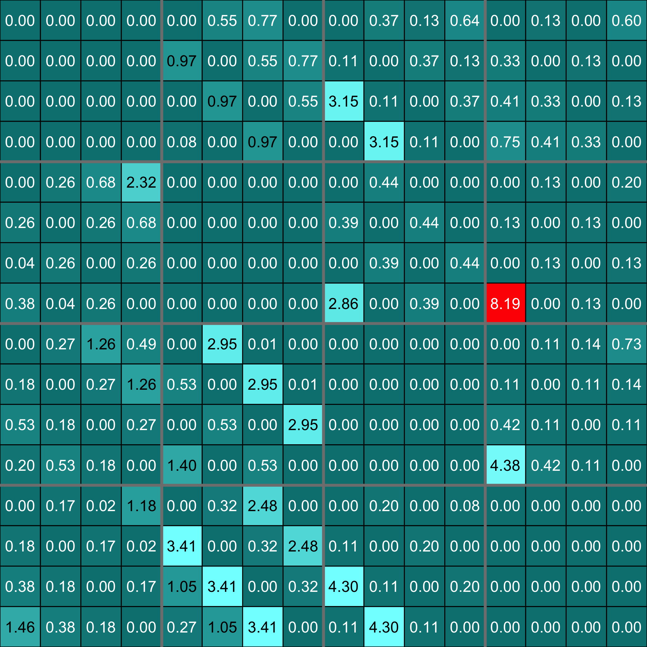
Plot the F matrix, for low dimensional F matrices.
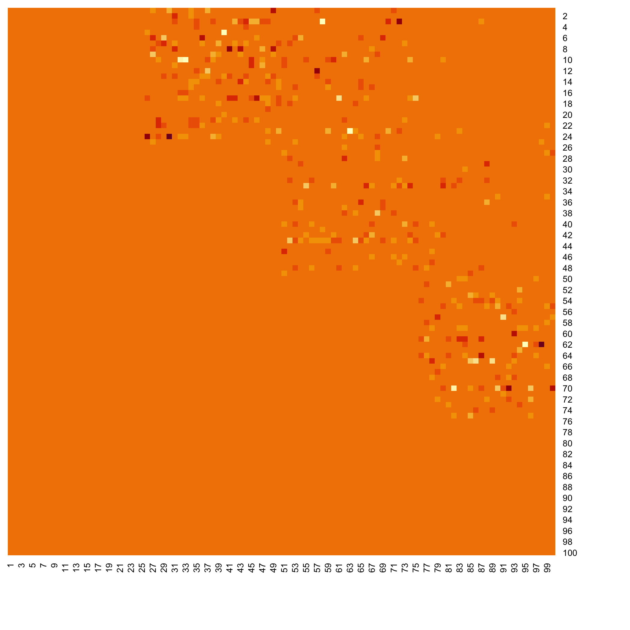
plot(Net, choice="F")
Plot the F matrix using the pixmap package, for high dimensional F matrices.
plot(Net, choice="Fpixmap")
We simulate gene expression according to the network that was previously drawn
set.seed(1)
M <- Patterns::gene_expr_simulation(
  network=Net,
  time_label=rep(1:4,each=25),
  subject=5,
  peak_level=200,
  act_time_group=1:4)
str(M)
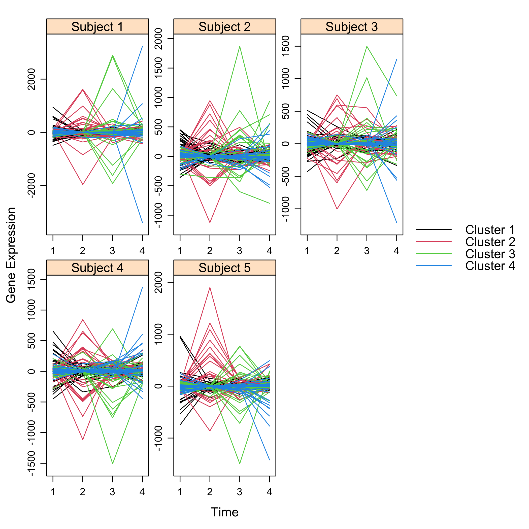
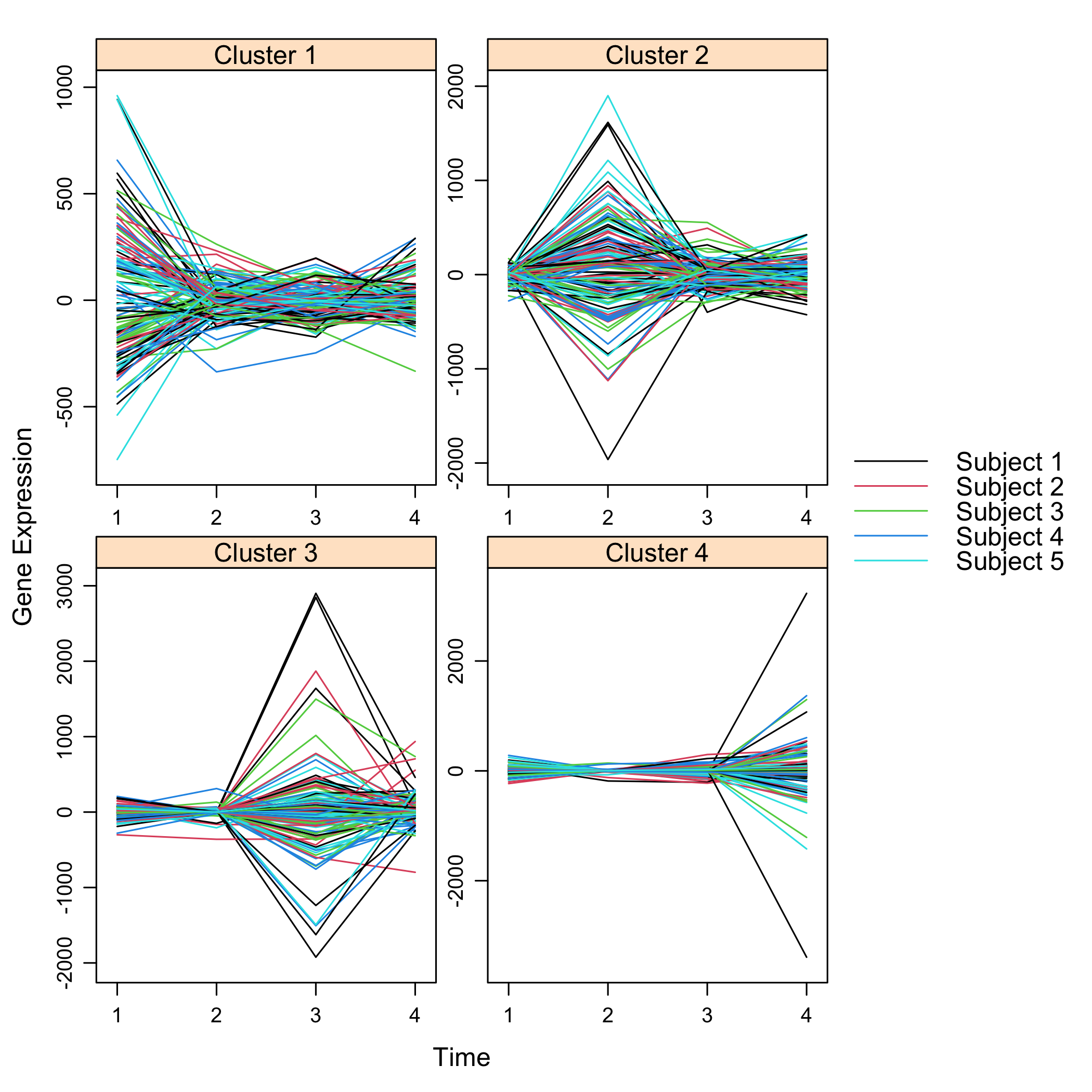
Get a summay and plots of the simulated data:
summary(M)
plot(M)
Network inferrence
We infer the new network using subjectwise leave one out cross-validation (default setting): all measurements from the same subject are removed from the dataset). The inference is carried out with a general Fshape.
Net_inf_P <- Patterns::inference(M, cv.subjects=TRUE)
Plot of the inferred F matrix
plot(Net_inf_P, choice="F")
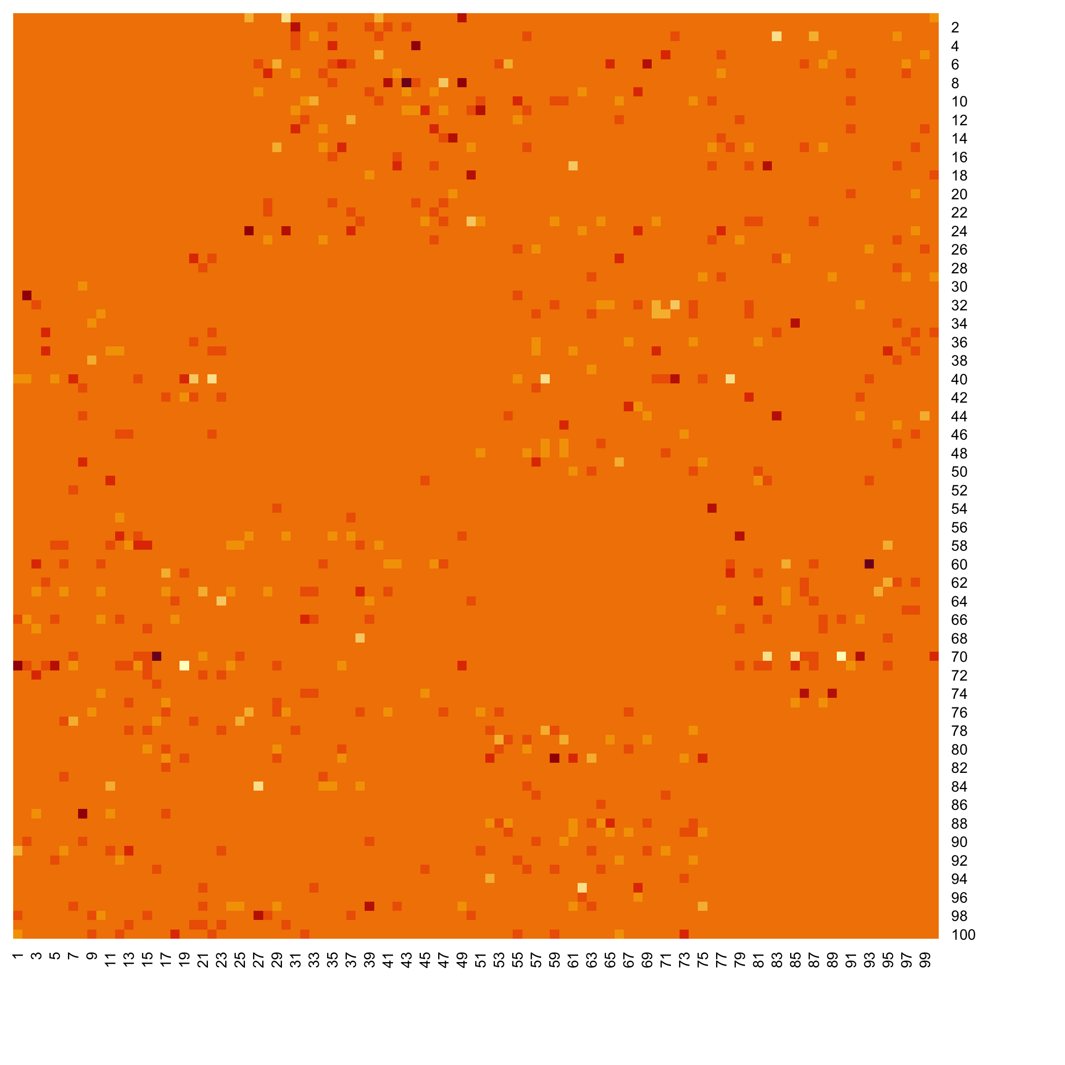
Heatmap of the inferred coefficients of the Omega matrix
stats::heatmap(Net_inf_P@network, Rowv = NA, Colv = NA, scale="none", revC=TRUE)
Default values fot the $F$ matrices. The Finit matrix (starting values for the algorithm). In our case, the Finitobject is an array of sizes $(T_i,T-i,Ngrp^2)=(4,4,16)$.
Ti<-4;
ngrp<-4
nF<-ngrp^2
Finit<-array(0,c(Ti,Ti,nF))
              for(ii in 1:nF){
                if((ii%%(ngrp+1))==1){
                  Finit[,,ii]<-0
                } else {
                  Finit[,,ii]<-cbind(rbind(rep(0,Ti-1),diag(1,Ti-1)),rep(0,Ti))+rbind(cbind(rep(0,Ti-1),diag(1,Ti-1)),rep(0,Ti))
                }
              }
The Fshape matrix (default shape for F matrix the algorithm). Any interaction between groups and times are permitted except the retro-actions (a group on itself, or an action at the same time for an actor on another one).
Fshape<-array("0",c(Ti,Ti,nF))
for(ii in 1:nF){
  if((ii%%(ngrp+1))==1){
    Fshape[,,ii]<-"0"
  } else {
    lchars <- paste("a",1:(2*Ti-1),sep="")
    tempFshape<-matrix("0",Ti,Ti)
    for(bb in (-Ti+1):(Ti-1)){
      tempFshape<-replaceUp(tempFshape,matrix(lchars[bb+Ti],Ti,Ti),-bb)
    }
    tempFshape <- replaceBand(tempFshape,matrix("0",Ti,Ti),0)
    Fshape[,,ii]<-tempFshape
  }
}
Any other form can be used. A "0" coefficient is missing from the model. It allows testing the best structure of an "F" matrix and even performing some significance tests of hypothses on the structure of the $F$ matrix.
The IndicFshape function allows to design custom F matrix for cascade networks with equally spaced measurements by specifying the zero and non zero $F_{ij}$ cells of the $F$ matrix. It is useful for models featuring several clusters of actors that are activated at the time. Let's define the following indicatrix matrix (action of all groups on each other, which is not a possible real modeling setting and is only used as an example):
TestIndic=matrix(!((1:(Ti^2))%%(ngrp+1)==1),byrow=TRUE,ngrp,ngrp)
TestIndic
For that choice, we get those init and shape $F$ matrices.
IndicFinit(Ti,ngrp,TestIndic)
IndicFshape(Ti,ngrp,TestIndic)
Those $F$ matrices are lower diagonal ones to enforce that an observed value at a given time can only be predicted by a value that was observed in the past only (i.e. neither at the same moment or in the future).
The plotF is convenient to display F matrices. Here are the the displays of the three $F$ matrices we have just introduced.
plotF(Fshape,choice="Fshape")
plotF(CascadeFshape(4,4),choice="Fshape")
plotF(IndicFshape(Ti,ngrp,TestIndic),choice="Fshape")
We now fit the model with an $F$ matrix that is designed for cascade networks.
Specific Fshape
Net_inf_P_S <- Patterns::inference(M, Finit=CascadeFinit(4,4), Fshape=CascadeFshape(4,4))
Plot of the inferred F matrix
plot(Net_inf_P_S, choice="F")
Heatmap of the coefficients of the Omega matrix of the network. They reflect the use of a special $F$ matrix. It is an example of an F matrix specifically designed to deal with cascade networks.
stats::heatmap(Net_inf_P_S@network, Rowv = NA, Colv = NA, scale="none", revC=TRUE)
There are many fitting functions provided with the Patterns package in order to search for specific features for the inferred network such as sparsity, robust links, high confidence links or stable through resampling links. :
- LASSO, from the
lars package
- LASSO2, from the
glmnet package. An unweighted and a weighted version of the algorithm are available
- SPLS, from the
spls package
- ELASTICNET, from the
elasticnet package
- stability.c060, from the
c060 package implementation of stability selection
- stability.c060.weighted, a new weighted version of the
c060 package implementation of stability selection
- robust, lasso from the
lars package with light random Gaussian noise added to the explanatory variables
- selectboost.weighted, a new weighted version of the
selectboost package implementation of the selectboost algorithm to look for the more stable links against resampling that takes into account the correlated structure of the predictors. If no weights are provided, equal weigths are for all the variables (=non weighted case).
Net_inf_P_Lasso2 <- Patterns::inference(M, Finit=CascadeFinit(4,4), Fshape=CascadeFshape(4,4), fitfun="LASSO2")
Plot of the inferred F matrix
plot(Net_inf_P_Lasso2, choice="F")
Heatmap of the coefficients of the Omega matrix of the network
stats::heatmap(Net_inf_P_Lasso2@network, Rowv = NA, Colv = NA, scale="none", revC=TRUE)
We create a weighting vector to perform weighted lasso inference.
Weights_Net=slot(Net,"network")
Weights_Net[Net@network!=0]=.1
Weights_Net[Net@network==0]=1000
Net_inf_P_Lasso2_Weighted <- Patterns::inference(M, Finit=CascadeFinit(4,4), Fshape=CascadeFshape(4,4), fitfun="LASSO2", priors=Weights_Net)
Plot of the inferred F matrix
plot(Net_inf_P_Lasso2_Weighted, choice="F")
Heatmap of the coefficients of the Omega matrix of the network
stats::heatmap(Net_inf_P_Lasso2_Weighted@network, Rowv = NA, Colv = NA, scale="none", revC=TRUE)
Net_inf_P_SPLS <- Patterns::inference(M, Finit=CascadeFinit(4,4), Fshape=CascadeFshape(4,4), fitfun="SPLS")
Plot of the inferred F matrix
plot(Net_inf_P_SPLS, choice="F")
Heatmap of the coefficients of the Omega matrix of the network
stats::heatmap(Net_inf_P_SPLS@network, Rowv = NA, Colv = NA, scale="none", revC=TRUE)
Net_inf_P_ELASTICNET <- Patterns::inference(M, Finit=CascadeFinit(4,4), Fshape=CascadeFshape(4,4), fitfun="ELASTICNET")
Plot of the inferred F matrix
plot(Net_inf_P_ELASTICNET, choice="F")
Heatmap of the coefficients of the Omega matrix of the network
stats::heatmap(Net_inf_P_ELASTICNET@network, Rowv = NA, Colv = NA, scale="none", revC=TRUE)
Net_inf_P_stability <- Patterns::inference(M, Finit=CascadeFinit(4,4), Fshape=CascadeFshape(4,4), fitfun="stability.c060")
Plot of the inferred F matrix
plot(Net_inf_P_stability, choice="F")
Heatmap of the coefficients of the Omega matrix of the network
stats::heatmap(Net_inf_P_stability@network, Rowv = NA, Colv = NA, scale="none", revC=TRUE)
Net_inf_P_StabWeight <- Patterns::inference(M, Finit=CascadeFinit(4,4), Fshape=CascadeFshape(4,4), fitfun="stability.c060.weighted", priors=Weights_Net)
Plot of the inferred F matrix
plot(Net_inf_P_StabWeight, choice="F")
Heatmap of the coefficients of the Omega matrix of the network
stats::heatmap(Net_inf_P_StabWeight@network, Rowv = NA, Colv = NA, scale="none", revC=TRUE)
Net_inf_P_Robust <- Patterns::inference(M, Finit=CascadeFinit(4,4), Fshape=CascadeFshape(4,4), fitfun="robust")
Plot of the inferred F matrix
plot(Net_inf_P_Robust, choice="F")
Heatmap of the coefficients of the Omega matrix of the network
stats::heatmap(Net_inf_P_Robust@network, Rowv = NA, Colv = NA, scale="none", revC=TRUE)
Weights_Net_1 <- Weights_Net
Weights_Net_1[,] <- 1
Net_inf_P_SelectBoost <- Patterns::inference(M, Finit=CascadeFinit(4,4), Fshape=CascadeFshape(4,4), fitfun="selectboost.weighted",priors=Weights_Net_1)
detach("package:Patterns", unload=TRUE)
library(Patterns)
Plot of the inferred F matrix
plot(Net_inf_P_SelectBoost, choice="F")
Heatmap of the coefficients of the Omega matrix of the network
stats::heatmap(Net_inf_P_SelectBoost@network, Rowv = NA, Colv = NA, scale="none", revC=TRUE)
Net_inf_P_SelectBoostWeighted <- Patterns::inference(M, Finit=CascadeFinit(4,4), Fshape=CascadeFshape(4,4), fitfun="selectboost.weighted",priors=Weights_Net)
detach("package:Patterns", unload=TRUE)
library(Patterns)
Plot of the inferred F matrix
plot(Net_inf_P_SelectBoostWeighted, choice="F")
Heatmap of the coefficients of the Omega matrix of the network
stats::heatmap(Net_inf_P_SelectBoostWeighted@network, Rowv = NA, Colv = NA, scale="none", revC=TRUE)
Post inference network analysis
Such an analysis is only required if the model was not fitted using the stability selection or the selectboost algorithm.
Create an animation of the network with increasing cutoffs with an animated .gif format or a html webpage in the working directory.
data(network)
sequence<-seq(0,0.2,length.out=20)
evolution(network,sequence,type.ani = "gif", outdir=getwd())
evolution(network,sequence,type.ani = "html", outdir=getwd())
data(network)
sequence<-seq(0,0.2,length.out=20)
#try(if(pkgdown::in_pkgdown()){destdir = "~/Github/Patterns/docs/reference/evolution/"})
destdir = "~/Github/Patterns/docs/reference/evolution/"
evolution(network,sequence,type.ani = "gif",outdir=destdir)
evolution(network,sequence,type.ani = "html",outdir=destdir)
Evolution of some properties of a reverse-engineered network with increasing cut-off values.
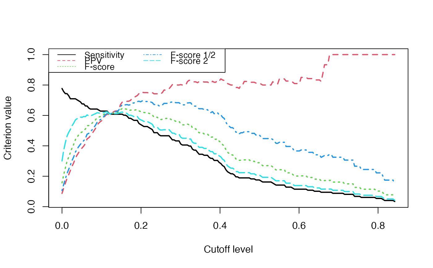
We switch to data that were derived from the inferrence of a real biological network and try to detect the optimal cutoff value: the best cutoff value for a network to fit a scale free network. The cutoff was validated only single group cascade networks (number of actors groups = number of timepoints) and for genes dataset. Instead of the cutoff function, manual curation or the stability selection or the selectboost algorithm should be used.
data("networkCascade")
set.seed(1)
cutoff(networkCascade)
Analyze the network with a cutoff set to the previouly found 0.133 optimal value.
analyze_network(networkCascade,nv=0.133)
data(Selection)
plot(networkCascade,nv=0.133, gr=Selection@group)
Perform gene selection
Import data.
library(Patterns)
library(CascadeData)
data(micro_S)
micro_S<-as.omics_array(micro_S,time=c(60,90,210,390),subject=6,gene_ID=rownames(micro_S))
data(micro_US)
micro_US<-as.omics_array(micro_US,time=c(60,90,210,390),subject=6,gene_ID=rownames(micro_US))
Select early genes (t1 or t2):
Selection1<-geneSelection(x=micro_S,y=micro_US,20,wanted.patterns=rbind(c(0,1,0,0),c(1,0,0,0),c(1,1,0,0)))
Section genes with first significant differential expression at t1:
Selection2<-geneSelection(x=micro_S,y=micro_US,20,peak=1)
Section genes with first significant differential expression at t2:
Selection3<-geneSelection(x=micro_S,y=micro_US,20,peak=2)
Select later genes (t3 or t4)
Selection4<-geneSelection(x=micro_S,y=micro_US,50,
wanted.patterns=rbind(c(0,0,1,0),c(0,0,0,1),c(1,1,0,0)))
Merge those selections:
Selection<-unionOmics(Selection1,Selection2)
Selection<-unionOmics(Selection,Selection3)
Selection<-unionOmics(Selection,Selection4)
head(Selection)
Summarize the final selection:
summary(Selection)
Plot the final selection:
plot(Selection)
This process could be improved by retrieve a real gene_ID using the bitr function of the ClusterProfiler package or by performing independent filtering using jetset package to only keep at most only probeset (the best one, if there is one good enough) per gene_ID.
Examples of outputs

fbertran/Patterns documentation built on Dec. 8, 2022, 8:48 p.m.
R Package Documentation
Browse R Packages
We want your feedback!
Note that we can't provide technical support on individual packages. You should contact the package authors for that.
knitr::opts_chunk$set( collapse = TRUE, comment = "#>", fig.path = "man/figures/README-", out.width = "100%", dpi=300,fig.width=7, fig.keep="all" )
Patterns
A modeling tool dedicated to biological network modeling to decipher Biological Networks with Patterned Heterogeneous (e.g. multiOmics) Measurements
Frédéric Bertrand and Myriam Maumy-Bertrand
![]()
![]()
![]()
![]()
It is designed to work with patterned data. Famous examples of problems related to patterned data are:
- recovering signals in networks after a stimulation (cascade network reverse engineering),
- analysing periodic signals.
It allows for single or joint modeling of, for instance, genes and proteins.
- It starts with the selection of the actors that will be the used in the reverse engineering upcoming step. An actor can be included in that selection based on its differential effects (for instance gene expression or protein abundance) or on its time course profile.
- Wrappers for actors clustering functions and cluster analysis are provided.
- It also allows reverse engineering of biological networks taking into account the observed time course patterns of the actors. Interactions between clusters of actors can be set by the user. Any number of clusters can be activated at a single time.
- Many inference functions are provided with the
Patternspackage and dedicated to get specific features for the inferred network such as sparsity, robust links, high confidence links or stable through resampling links.- lasso, from the
larspackage - lasso, from the
glmnetpackage. An unweighted and a weighted version of the algorithm are available - spls, from the
splspackage - elasticnet, from the
elasticnetpackage - stability selection, from the
c060package implementation of stability selection - weighted stability selection, a new weighted version of the
c060package implementation of stability selection that I created for the package - robust, lasso from the
larspackage with light random Gaussian noise added to the explanatory variables - selectboost, from the
selectboostpackage. The selectboost algorithm looks for the more stable links against resampling that takes into account the correlated structure of the predictors - weighted selectboost, a new weighted version of the
selectboost.
- lasso, from the
- Some simulation and prediction tools are also available for cascade networks.
- Examples of use with microarray or RNA-Seq data are provided.
The weights are viewed as a penalty factors in the penalized regression model: it is a number that multiplies the lambda value in the minimization problem to allow differential shrinkage, Friedman et al. 2010, equation 1 page 3. If equal to 0, it implies no shrinkage, and that variable is always included in the model. Default is 1 for all variables. Infinity means that the variable is excluded from the model. Note that the weights are rescaled to sum to the number of variables.
A word for those that have been using our seminal work, the Cascade package that we created several years ago and that was a very efficient network reverse engineering tool for cascade networks
(Jung, N., Bertrand, F., Bahram, S., Vallat, L., and Maumy-Bertrand, M. (2014), https://doi.org/10.1093/bioinformatics/btt705, https://cran.r-project.org/package=Cascade, https://github.com/fbertran/Cascade and https://fbertran.github.io/Cascade/).
The Patterns package is more than (at least) a threeway major extension of the Cascade package :
- any number of groups can be used whereas in the
Cascadepackage only 1 group for each timepoint could be created, which prevented the users to create homogeneous clusters of genes in datasets that featured more than a few dozens of genes. - custom $F$ matrices shapes whereas in the
Cascadepackage only 1 shape was provided:- interaction between groups
- custom design of inner cells of the $F$ matrix
- the custom $F$ matrices allow to deal with heteregeneous networks with several kinds of actors such as mixing genes and proteins in a single network to perform joint inference.
- about nine inference algorithms are provided, whereas 1 (lasso) in
Cascade.
Hence the Patterns package should be viewed more as a completely new modelling tools than as an extension of the Cascade package.
This website and these examples were created by F. Bertrand and M. Maumy-Bertrand.
Installation
You can install the released version of Patterns from CRAN with:
install.packages("Patterns")
You can install the development version of Patterns from github with:
devtools::install_github("fbertran/Patterns")
Examples
Data management
Import Cascade Data (repeated measurements on several subjects) from the CascadeData package and turn them into a omics array object. The second line makes sure the CascadeData package is installed.
library(Patterns)
if(!require(CascadeData)){install.packages("CascadeData")} data(micro_US) micro_US<-as.omics_array(micro_US[1:100,],time=c(60,90,210,390),subject=6) str(micro_US)
Get a summay and plots of the data:
summary(micro_US) plot(micro_US)
Gene selection
There are several functions to carry out gene selection before the inference. They are detailed in the vignette of the package.
Data simulation
Let's simulate some cascade data and then do some reverse engineering.
We first design the F matrix for $T_i=4$ times and $Ngrp=4$ groups. The Fmatobject is an array of sizes $(T_i,T-i,Ngrp^2)=(4,4,16)$.
Ti<-4 Ngrp<-4 Fmat=array(0,dim=c(Ti,Ti,Ngrp^2)) for(i in 1:(Ti^2)){ if(((i-1) %% Ti) > (i-1) %/% Ti){ Fmat[,,i][outer(1:Ti,1:Ti,function(x,y){0<(x-y) & (x-y)<2})]<-1 } }
The Patterns function CascadeFinit is an utility function to easily define such an F matrix.
Fbis=Patterns::CascadeFinit(Ti,Ngrp,low.trig=FALSE) str(Fbis)
Check if the two matrices Fmat and Fbis are identical.
print(all(Fmat==Fbis))
End of F matrix definition.
Fmat[,,3]<-Fmat[,,3]*0.2 Fmat[3,1,3]<-1 Fmat[4,2,3]<-1 Fmat[,,4]<-Fmat[,,3]*0.3 Fmat[4,1,4]<-1 Fmat[,,8]<-Fmat[,,3]
We set the seed to make the results reproducible and draw a scale free random network.
set.seed(1) Net<-Patterns::network_random( nb=100, time_label=rep(1:4,each=25), exp=1, init=1, regul=round(rexp(100,1))+1, min_expr=0.1, max_expr=2, casc.level=0.4 ) Net@F<-Fmat str(Net)
Plot the simulated network.
Patterns::plot(Net, choice="network")
If a gene clustering is known, it can be used as a coloring scheme.
plot(Net, choice="network", gr=rep(1:4,each=25))
Plot the F matrix, for low dimensional F matrices.
plot(Net, choice="F")
Plot the F matrix using the pixmap package, for high dimensional F matrices.
plot(Net, choice="Fpixmap")
We simulate gene expression according to the network that was previously drawn
set.seed(1) M <- Patterns::gene_expr_simulation( network=Net, time_label=rep(1:4,each=25), subject=5, peak_level=200, act_time_group=1:4) str(M)
Get a summay and plots of the simulated data:
summary(M)
plot(M)
Network inferrence
We infer the new network using subjectwise leave one out cross-validation (default setting): all measurements from the same subject are removed from the dataset). The inference is carried out with a general Fshape.
Net_inf_P <- Patterns::inference(M, cv.subjects=TRUE)
Plot of the inferred F matrix
plot(Net_inf_P, choice="F")
Heatmap of the inferred coefficients of the Omega matrix
stats::heatmap(Net_inf_P@network, Rowv = NA, Colv = NA, scale="none", revC=TRUE)
Default values fot the $F$ matrices. The Finit matrix (starting values for the algorithm). In our case, the Finitobject is an array of sizes $(T_i,T-i,Ngrp^2)=(4,4,16)$.
Ti<-4; ngrp<-4 nF<-ngrp^2 Finit<-array(0,c(Ti,Ti,nF)) for(ii in 1:nF){ if((ii%%(ngrp+1))==1){ Finit[,,ii]<-0 } else { Finit[,,ii]<-cbind(rbind(rep(0,Ti-1),diag(1,Ti-1)),rep(0,Ti))+rbind(cbind(rep(0,Ti-1),diag(1,Ti-1)),rep(0,Ti)) } }
The Fshape matrix (default shape for F matrix the algorithm). Any interaction between groups and times are permitted except the retro-actions (a group on itself, or an action at the same time for an actor on another one).
Fshape<-array("0",c(Ti,Ti,nF)) for(ii in 1:nF){ if((ii%%(ngrp+1))==1){ Fshape[,,ii]<-"0" } else { lchars <- paste("a",1:(2*Ti-1),sep="") tempFshape<-matrix("0",Ti,Ti) for(bb in (-Ti+1):(Ti-1)){ tempFshape<-replaceUp(tempFshape,matrix(lchars[bb+Ti],Ti,Ti),-bb) } tempFshape <- replaceBand(tempFshape,matrix("0",Ti,Ti),0) Fshape[,,ii]<-tempFshape } }
Any other form can be used. A "0" coefficient is missing from the model. It allows testing the best structure of an "F" matrix and even performing some significance tests of hypothses on the structure of the $F$ matrix.
The IndicFshape function allows to design custom F matrix for cascade networks with equally spaced measurements by specifying the zero and non zero $F_{ij}$ cells of the $F$ matrix. It is useful for models featuring several clusters of actors that are activated at the time. Let's define the following indicatrix matrix (action of all groups on each other, which is not a possible real modeling setting and is only used as an example):
TestIndic=matrix(!((1:(Ti^2))%%(ngrp+1)==1),byrow=TRUE,ngrp,ngrp) TestIndic
For that choice, we get those init and shape $F$ matrices.
IndicFinit(Ti,ngrp,TestIndic) IndicFshape(Ti,ngrp,TestIndic)
Those $F$ matrices are lower diagonal ones to enforce that an observed value at a given time can only be predicted by a value that was observed in the past only (i.e. neither at the same moment or in the future).
The plotF is convenient to display F matrices. Here are the the displays of the three $F$ matrices we have just introduced.
plotF(Fshape,choice="Fshape")
plotF(CascadeFshape(4,4),choice="Fshape")
plotF(IndicFshape(Ti,ngrp,TestIndic),choice="Fshape")
We now fit the model with an $F$ matrix that is designed for cascade networks.
Specific Fshape
Net_inf_P_S <- Patterns::inference(M, Finit=CascadeFinit(4,4), Fshape=CascadeFshape(4,4))
Plot of the inferred F matrix
plot(Net_inf_P_S, choice="F")
Heatmap of the coefficients of the Omega matrix of the network. They reflect the use of a special $F$ matrix. It is an example of an F matrix specifically designed to deal with cascade networks.
stats::heatmap(Net_inf_P_S@network, Rowv = NA, Colv = NA, scale="none", revC=TRUE)
There are many fitting functions provided with the Patterns package in order to search for specific features for the inferred network such as sparsity, robust links, high confidence links or stable through resampling links. :
- LASSO, from the
larspackage - LASSO2, from the
glmnetpackage. An unweighted and a weighted version of the algorithm are available - SPLS, from the
splspackage - ELASTICNET, from the
elasticnetpackage - stability.c060, from the
c060package implementation of stability selection - stability.c060.weighted, a new weighted version of the
c060package implementation of stability selection - robust, lasso from the
larspackage with light random Gaussian noise added to the explanatory variables - selectboost.weighted, a new weighted version of the
selectboostpackage implementation of the selectboost algorithm to look for the more stable links against resampling that takes into account the correlated structure of the predictors. If no weights are provided, equal weigths are for all the variables (=non weighted case).
Net_inf_P_Lasso2 <- Patterns::inference(M, Finit=CascadeFinit(4,4), Fshape=CascadeFshape(4,4), fitfun="LASSO2")
Plot of the inferred F matrix
plot(Net_inf_P_Lasso2, choice="F")
Heatmap of the coefficients of the Omega matrix of the network
stats::heatmap(Net_inf_P_Lasso2@network, Rowv = NA, Colv = NA, scale="none", revC=TRUE)
We create a weighting vector to perform weighted lasso inference.
Weights_Net=slot(Net,"network") Weights_Net[Net@network!=0]=.1 Weights_Net[Net@network==0]=1000
Net_inf_P_Lasso2_Weighted <- Patterns::inference(M, Finit=CascadeFinit(4,4), Fshape=CascadeFshape(4,4), fitfun="LASSO2", priors=Weights_Net)
Plot of the inferred F matrix
plot(Net_inf_P_Lasso2_Weighted, choice="F")
Heatmap of the coefficients of the Omega matrix of the network
stats::heatmap(Net_inf_P_Lasso2_Weighted@network, Rowv = NA, Colv = NA, scale="none", revC=TRUE)
Net_inf_P_SPLS <- Patterns::inference(M, Finit=CascadeFinit(4,4), Fshape=CascadeFshape(4,4), fitfun="SPLS")
Plot of the inferred F matrix
plot(Net_inf_P_SPLS, choice="F")
Heatmap of the coefficients of the Omega matrix of the network
stats::heatmap(Net_inf_P_SPLS@network, Rowv = NA, Colv = NA, scale="none", revC=TRUE)
Net_inf_P_ELASTICNET <- Patterns::inference(M, Finit=CascadeFinit(4,4), Fshape=CascadeFshape(4,4), fitfun="ELASTICNET")
Plot of the inferred F matrix
plot(Net_inf_P_ELASTICNET, choice="F")
Heatmap of the coefficients of the Omega matrix of the network
stats::heatmap(Net_inf_P_ELASTICNET@network, Rowv = NA, Colv = NA, scale="none", revC=TRUE)
Net_inf_P_stability <- Patterns::inference(M, Finit=CascadeFinit(4,4), Fshape=CascadeFshape(4,4), fitfun="stability.c060")
Plot of the inferred F matrix
plot(Net_inf_P_stability, choice="F")
Heatmap of the coefficients of the Omega matrix of the network
stats::heatmap(Net_inf_P_stability@network, Rowv = NA, Colv = NA, scale="none", revC=TRUE)
Net_inf_P_StabWeight <- Patterns::inference(M, Finit=CascadeFinit(4,4), Fshape=CascadeFshape(4,4), fitfun="stability.c060.weighted", priors=Weights_Net)
Plot of the inferred F matrix
plot(Net_inf_P_StabWeight, choice="F")
Heatmap of the coefficients of the Omega matrix of the network
stats::heatmap(Net_inf_P_StabWeight@network, Rowv = NA, Colv = NA, scale="none", revC=TRUE)
Net_inf_P_Robust <- Patterns::inference(M, Finit=CascadeFinit(4,4), Fshape=CascadeFshape(4,4), fitfun="robust")
Plot of the inferred F matrix
plot(Net_inf_P_Robust, choice="F")
Heatmap of the coefficients of the Omega matrix of the network
stats::heatmap(Net_inf_P_Robust@network, Rowv = NA, Colv = NA, scale="none", revC=TRUE)
Weights_Net_1 <- Weights_Net Weights_Net_1[,] <- 1 Net_inf_P_SelectBoost <- Patterns::inference(M, Finit=CascadeFinit(4,4), Fshape=CascadeFshape(4,4), fitfun="selectboost.weighted",priors=Weights_Net_1)
detach("package:Patterns", unload=TRUE) library(Patterns)
Plot of the inferred F matrix
plot(Net_inf_P_SelectBoost, choice="F")
Heatmap of the coefficients of the Omega matrix of the network
stats::heatmap(Net_inf_P_SelectBoost@network, Rowv = NA, Colv = NA, scale="none", revC=TRUE)
Net_inf_P_SelectBoostWeighted <- Patterns::inference(M, Finit=CascadeFinit(4,4), Fshape=CascadeFshape(4,4), fitfun="selectboost.weighted",priors=Weights_Net)
detach("package:Patterns", unload=TRUE) library(Patterns)
Plot of the inferred F matrix
plot(Net_inf_P_SelectBoostWeighted, choice="F")
Heatmap of the coefficients of the Omega matrix of the network
stats::heatmap(Net_inf_P_SelectBoostWeighted@network, Rowv = NA, Colv = NA, scale="none", revC=TRUE)
Post inference network analysis
Such an analysis is only required if the model was not fitted using the stability selection or the selectboost algorithm.
Create an animation of the network with increasing cutoffs with an animated .gif format or a html webpage in the working directory.
data(network) sequence<-seq(0,0.2,length.out=20) evolution(network,sequence,type.ani = "gif", outdir=getwd()) evolution(network,sequence,type.ani = "html", outdir=getwd())
data(network) sequence<-seq(0,0.2,length.out=20) #try(if(pkgdown::in_pkgdown()){destdir = "~/Github/Patterns/docs/reference/evolution/"}) destdir = "~/Github/Patterns/docs/reference/evolution/" evolution(network,sequence,type.ani = "gif",outdir=destdir) evolution(network,sequence,type.ani = "html",outdir=destdir)
Evolution of some properties of a reverse-engineered network with increasing cut-off values.
We switch to data that were derived from the inferrence of a real biological network and try to detect the optimal cutoff value: the best cutoff value for a network to fit a scale free network. The cutoff was validated only single group cascade networks (number of actors groups = number of timepoints) and for genes dataset. Instead of the cutoff function, manual curation or the stability selection or the selectboost algorithm should be used.
data("networkCascade") set.seed(1) cutoff(networkCascade)
Analyze the network with a cutoff set to the previouly found 0.133 optimal value.
analyze_network(networkCascade,nv=0.133)
data(Selection) plot(networkCascade,nv=0.133, gr=Selection@group)
Perform gene selection
Import data.
library(Patterns) library(CascadeData) data(micro_S) micro_S<-as.omics_array(micro_S,time=c(60,90,210,390),subject=6,gene_ID=rownames(micro_S)) data(micro_US) micro_US<-as.omics_array(micro_US,time=c(60,90,210,390),subject=6,gene_ID=rownames(micro_US))
Select early genes (t1 or t2):
Selection1<-geneSelection(x=micro_S,y=micro_US,20,wanted.patterns=rbind(c(0,1,0,0),c(1,0,0,0),c(1,1,0,0)))
Section genes with first significant differential expression at t1:
Selection2<-geneSelection(x=micro_S,y=micro_US,20,peak=1)
Section genes with first significant differential expression at t2:
Selection3<-geneSelection(x=micro_S,y=micro_US,20,peak=2)
Select later genes (t3 or t4)
Selection4<-geneSelection(x=micro_S,y=micro_US,50, wanted.patterns=rbind(c(0,0,1,0),c(0,0,0,1),c(1,1,0,0)))
Merge those selections:
Selection<-unionOmics(Selection1,Selection2) Selection<-unionOmics(Selection,Selection3) Selection<-unionOmics(Selection,Selection4) head(Selection)
Summarize the final selection:
summary(Selection)
Plot the final selection:
plot(Selection)
This process could be improved by retrieve a real gene_ID using the bitr function of the ClusterProfiler package or by performing independent filtering using jetset package to only keep at most only probeset (the best one, if there is one good enough) per gene_ID.
Examples of outputs
R Package Documentation
Browse R Packages
We want your feedback!
Note that we can't provide technical support on individual packages. You should contact the package authors for that.
Embedding an R snippet on your website
Add the following code to your website.
For more information on customizing the embed code, read Embedding Snippets.