README.md

In hzhang0311/lmcoef: Coefficients Estimation for Fitted Model

lmcoef

Overview

lmcoef is a package for statistical analysis that allows users to obtain estimation results from linear regression model with another implementation. As a substitution for the well-known lm function, this package aims to allow users to separately obtain different estimates that are more useful for them adjusting for different scenarios when analyzing larger data sets. As a new implementation, it would save much time when user facing a specific condition of constraint polynomial regression.

So far, this package includes one function:

• lm_coef(): Compute estimated coefficients of linear regression model with testing results, and returns alongside with ANOVA table, R squared, adjusted R squared, values of fitted values and residuals.

• cpr_coef(): Compute estimated coefficients of constraint polynomial regression model with testing results, and returns alongside with values of fitted values and residuals. The function is applicable if and only if the constraint is:

For i = 1,...,n

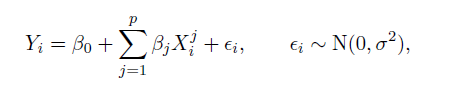
where parameter beta(j) = beta(j-1)/j for j = 2,...,p and predictor X(i) = i/n.

Installation

Github installation is used to install lmcoef:

# install.packages("devtools")
devtools::install_github("hzhang0311/lmcoef")

Usage

## SKIP: Download & Installation
# install.packages("devtools")
# devtools::install_github("hzhang0311/lmcoef")
library(lmcoef)

######################## lm_coef ########################
## Given the data below
y = c(78.5, 74.3, 104.3, 87.6, 95.9, 109.2, 102.7, 72.5, 93.1, 115.9, 83.8, 113.3, 109.4)
x = data.frame(X1 = c(7, 1, 11, 11, 7, 11, 3, 1, 2, 21, 1, 11, 10), 
               X2 = c(26, 29, 56, 31, 52, 55, 71, 31, 54, 47, 40, 66, 68), 
               X3 = c(6, 15, 8, 8, 6, 9, 17, 22, 18, 4, 23, 9, 8), 
               X4 = c(60, 52, 20, 47, 33, 22, 6, 44, 22, 26, 34, 12, 12))

# To obatin both estimated coefficients and quantiled residuals
rst = lm_coef(y,x)

# To obatin estimated coefficients alone
rst$coefficients

# >               Estimate    Std_Err     t.stat    p.value
# > (intercept) 62.4053693 70.0709592  0.8906025 0.39913356
# > X1           1.5511026  0.7447699  2.0826603 0.07082169
# > X2           0.5101676  0.7237880  0.7048577 0.50090110
# > X3           0.1019094  0.7547090  0.1350314 0.89592269
# > X4          -0.1440610  0.7090521 -0.2031741 0.84407147

# To obtain the ANOVA table
rst$anova

# >           Df       Sum.Sq      Mean.Sq      F.value      p.value
# > X1         1 1450.0763281 1450.0763281 242.36791816 2.887559e-07
# > X2         1 1207.7822656 1207.7822656 201.87052753 5.863323e-07
# > X3         1    9.7938691    9.7938691   1.63696188 2.366003e-01
# > X4         1    0.2469747    0.2469747   0.04127972 8.440715e-01
# > Residuals  8   47.8636394    5.9829549           NA           NA

# To obatin R squared, adjusted R squared, residuals, or fitted values alone
rst$R2    # > [1] 0.9823756
rst$R2_adj    # > [1] 0.9735634

rst$residuals
# >           [,1]
# > [1,]  0.004760419
# > [2,]  1.511200700
# > [3,] -1.670937532
# > [4,] -1.727100255
# > [5,]  0.250755562
# > [6,]  3.925442702
# > [7,] -1.448669087
# > [8,] -3.174988517
# > [9,]  1.378349477
# > [10,]  0.281547999
# > [11,]  1.990983571
# > [12,]  0.972989035
# > [13,] -2.294334073

rst$fitted.values
# >           [,1]
# > [1,]  78.49524
# > [2,]  72.78880
# > [3,] 105.97094
# > [4,]  89.32710
# > [5,]  95.64924
# > [6,] 105.27456
# > [7,] 104.14867
# > [8,]  75.67499
# > [9,]  91.72165
# > [10,] 115.61845
# > [11,]  81.80902
# > [12,] 112.32701
# > [13,] 111.69433


######################## cpr_coef ########################
# Given the data as below
p = 5
y = c(1,3,3,3,4,5,3,2,-1)

cpr_coef(p, y)

# > $coefficients
# >                 Estimate
# > (intercept)  3.452393951
# > b1          -1.100167971
# > b2          -0.550083985
# > b3          -0.183361328
# > b4          -0.045840332
# > b5          -0.009168066
# > 
# > $fitted.values
# > [1] 3.323103 3.178619 3.017156 2.836727 2.635118 2.409875 2.158283 1.877347 1.563772
# > 
# > $residuals
# > [1]  2.32310324  0.17861859  0.01715603 -0.16327333 -1.36488198 -2.59012461 -0.84171677 -0.12265344  2.56377227

# To obtain the results separately
cpr_res = cpr_coef(p, y)

cpr_res$coefficients

# >                 Estimate
# > (intercept)  3.452393951
# > b1          -1.100167971
# > b2          -0.550083985
# > b3          -0.183361328
# > b4          -0.045840332
# > b5          -0.009168066

cpr_res$residuals
# > [1]  2.32310324  0.17861859  0.01715603 -0.16327333 -1.36488198 -2.59012461 -0.84171677 -0.12265344  2.56377227

cpr_res$fitted.values
# > [1] 3.323103 3.178619 3.017156 2.836727 2.635118 2.409875 2.158283 1.877347 1.563772

hzhang0311/lmcoef documentation built on Dec. 20, 2021, 5:55 p.m.