README.md

In sysbiosig/SCRC: Fractional response analysis

Fractional Response Analysis (FRA) - R package

R- package FRA is designed to perform fractional response analysi of single-cell responses as presented in the manuscript Nienałtowski et al. "Fractional response analysis reveals logarithmic cytokine responses in cellular populations" Submitted (2020). A comprehensive documentation is available in directory Manual.pdf. In the folder 'article' you can find scripts for computing FRA for datasets described in the manuscript.

Setup

## Requirements - Hardware + A 32 or 64 bit processor (recommended: 64bit) + 1GHz processor (recommended: multicore for a comprehensive analysis) + 2GB MB RAM (recommended: 4GB+, depends on the size of experimental data)

Requirements - Software

The main software requirement is the installation of the R environment (version: >= 3.2), which can be downloaded from R project website and is distributed for all common operating systems. We tested the package in R environment installed on Windows 7, 10; Mac OS X 10.11 - 10.13 and Ubuntu 18.04 with no significant differences in the performance. The use of a dedicated Integrated development environment (IDE), e.g. RStudio is recommended.

Apart from a base installation of R, SLEMI requires the following R packages:

1. for installation

2. devtools

3. for estimation

4. nnet

5. doParallel

6. for visualisation

7. ggplot2

8. ggthemes
9. grDevices

10. viridis

11. for data handling

12. data.table

13. reshape2
14. dplyr
15. foreach

Each of the above packages can be installed by executing

install.packages("name_of_a_package")

in the R console.

Importantly, during installation availability of the above packages will be verified and missing packages will be automatically installed. Installation of the software and R packages takes ~1-2 hours.

Installation

The package can be directly installed from GitHub. For installation, open RStudio (or base R) and run following commands in the R console

# install.packages("devtools") # run if not installed

library(devtools)

install_github("sysbiosig/FRA")

All packages that are required will be installed or updated automatically. Installation of FRA package take ~ 5 minutes.

Basic usage

The FRA package provides their functionalities with three main functions:

1. FRA()- fractional response analysis performed for heterogeneous, multivariate, and dynamic measurements. Function computes: (i) the fractional response curve (FRC) that quantifies fractions of cells that exhibit different responses to a change in dose, or any other experimental conditionand and (ii) the cell-to-cell heterogeneity, i.e.fraction of cells exposed to one dose that exhibits responses in the range characteristic for other doses.

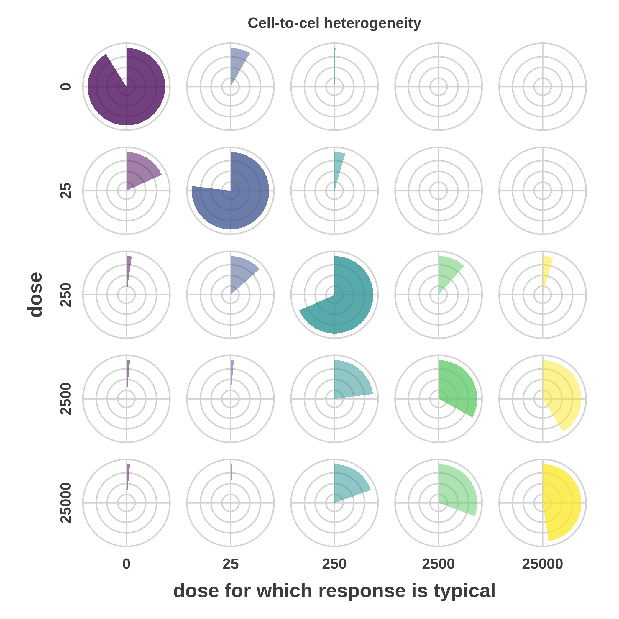
2. plotHeterogeneityPieCharts() - visualises the cell-to-cell heterogeneity structure using table of pie charts. Each pie chart describes the fraction of cells exposed to one dose (rows) that expibits responses typical for either of the doses (columns).

3. plotFRC()- visualises FRC and the cell-to-cell heterogenity. FRC is represented as a line, whereas heterogeneity is represented as colour band.

Morevoer, package contains examplary datasets, that were used in the publication:

1. data.fra.cytof - only part that describe responses of monocytes CD14+

2. data.fra.ps1

3. data.fra.ps3

4. data.fra.nfkb

Preaparing data

The function FRA() takes data in the form of the object data.frame with a specifc structure of rows and columns. Responses $y^i_j$ are assumed to be measured for a finite set of stimuli levels $x_1,x_2,\ldots,x_m$. The responses $y^i_j$ can be multidimensional.

Example of usage

Below, we present an application of FRA package to the case of the multivariate dose-responses to IFN-a2a in monocytes CD14+ described in the article. Fractional response analysis are computed by calling function: ```{r scrc_cytof_1, include=FALSE, cache=TRUE, eval=TRUE }

library(FRA) model <- FRA( data = FRA::data.fra.cytof, signal = "Stim", response = c("pSTAT1", "pSTAT3", "pSTAT4", "pSTAT5", "pSTAT6"), parallel_cores = 1, bootstrap.number = 32)

Time of the computations strongly depends on number of bootstrap samples specified by parameter `bootstrap.number`. Here, for `bootstrap.number == 32`, computation have taken ~10 minutes. The result is called by:
```{r scrc_cytof_2, include=TRUE, eval=TRUE }
> print(model)
FRAModel 
formula : Stim ~ pSTAT1+pSTAT3+pSTAT4+pSTAT5+pSTAT6 
FRA : 
    0    25   250  2500 25000 
 1.00  1.73  2.52  3.10  3.17 
confusion matrix : 
         0   25  250 2500 25000
0     0.91 0.08 0.00 0.00  0.00
25    0.19 0.77 0.05 0.00  0.00
250   0.02 0.14 0.68 0.11  0.05
2500  0.01 0.01 0.23 0.34  0.40
25000 0.01 0.01 0.19 0.31  0.47

To plot fractional response curve call: ```{r scrc_cytof_3, include=TRUE, eval=TRUE, cache=TRUE }

FRA::plotFRC(model = model)

![Fractional response curve](https://github.com/sysbiosig/FRA/blob/master/FRA_frc.png?raw=true)

To obtain the cell-to-cell heterogeneity as a pie charts call:
```{r scrc_cytof_4, include=TRUE, eval=TRUE, cache=TRUE }
> FRA::plotHeterogeneityPieCharts(model = model)

Documentation

Fractional response analysis

In order to perform fractional response analysis of single-cell data call

model <-FRA(
  data,
  signal = "signal",
  response = "response",
  sample = "sample",
  bootstrap.number = 0,
  bootstrap.sample_size = 1000,
  parallel_cores = 1,
  lr_maxit = 1000,
  MaxNWts = 5000,
  ...
)

``````

The required arguments are:

* `data` - a data.frame or data.table object in a wide format that describe response (might be multidimmensional) of the samples to the signal (one dimmensional, numeric); data.frame data consists numeric columns of names defined by signal, response,  and sample (optional); each row represents a response of one sample to the input signal; column signal define the input signal; columns response define the multidimmensional response to the input signal; column sample specify identifaction of sample; if sample is not defined then sample is identified by a row number; 
* `signal` - character, specify name of the column that represents the input signal;    
* `response` vector of characters, that specify names of the columns that represents the output response;
* `sample`  - character (optional), specify name of the column that consists identifiaction of sample;
* `parallel_cores` - specify number of cores used for computations, `default = 1`
* `bootstrap.number` (`default = 1`) - numeric, `bootstrap.number >= 1`, specify number of bootstrap samples used for estimation FRC and cell-to-cell heterogeneity. It is crucial to choose this value carefully, as it induce estimator accuracy. The proper value depends on data dimmensions and density distribution. The practice indicates that the higher number of bootstrap samples are required to obtain satisfying level of the accuracy of the cell-to-cell heterogeneity estimator. The `bootstrap.number = 1` denotes that one bootstrap sampling is performed to guarantee equipotence between number of cells for each dose, that is assumed in method;
*  `bootstrap.sample_size` (`default = 1000`) - numeric, size of the bootstrap sample;
* `lr_maxit` (`default = 1000`) - a maximum number of iterations of fitting step of logistic regression algorithm in `nnet` function. If a warning regarding lack of convergence of logistic model occurs, should be set to a larger value (possible if data is more complex or of a very high dimension); 
* `MaxNWts` (`default = 5000`) - a maximum number of parameters in logistic regression model. A limit is set to prevent accidental over-loading the memory. It should be set to a larger value in case of exceptionally high dimension of the output data or very high number of input values. In principle, logistic model requires fitting $(m-1)\cdot(d+1)$ parameters, where $m$ is the number of unique input values and $d$ is the dimension of the output.

The function returns the `FRAModel` object that contains among others
* `frc` - a `data.frame` that describe fractional response curve; contains two columns `dose` and `frc`
* `heterogeneity` - a `data.frame` that describes cell-to-cell heterogeneity, i.e., fraction of cells exposed to one dose (rows) that exhibits responses in the range characteristic for other doses (columns).

## Fractional Response Curve 
In order to visualise fractional response curve call 
```c
plotFRC(
    model,
    title_ =
      "Fractional Response Curve",
    xlab_ = "Dose",
    ylab_ = "Cumulative fraction of cells",
    fill.guide_ = "legend",
    ylimits_ = TRUE,
    alpha_ = 0.5,
    theme.signal = NULL,
    plot.heterogeneity = TRUE,
    ...

• model - FRAModel object return by FRA function
• title_ - character, specify title of plot, default "Fractional Response Curve"
• xlab_ - character, label of x axes, default "Dose"
• ylab_ - character, label of y axes and legend title, default "Cumulative fraction of cells"
• fill.guide_ - argument specify if legend should be displayed; legend is displayed for fill.guide_ = "legend", legend is not displayed for fill.guide_ = NULL, default = "legend"
• ylimits_ - logical (TRUE or FALSE) or numeric vector of minimum and maximum of y axes,
• theme.signal - optional, object returned by GetRescaledSignalTheme
• plot.heterogeneity - logical, define if FRC visualise the heterogeneity structure, default = TRUE

Cell-to-cell heterogeneity structure

In order to visualise th cell-to-cell heterogeneity structure, call

plotHeterogeneityPieCharts(
  model,
  max.signal = NULL,
  title_ = "Cell-to-cel heterogeneity",
  ylab_ = "dose",
  xlab_ = "dose for which response is typical",
  ...
)

• model - FRAModel object return by FRA function
• max.signal - maximal signal for which the cell-to-cell heterogeneity is plotted, default = max(signal)
• title_ - character, specify title of plot, default = "Cell-to-cel heterogeneity"
• ylab_ - character, label of y axes, default = "dose"
• xlab_ - character, label of x axes, default = "dose for which response is typical"

Citation

The package implements methods described in the article:

Nienałtowski K, Rigby R.E., Walczak J., Zakrzewska K.E., Rehwinkel J, and Komorowski M (2020) Fractional response analysis reveals logarithmic cytokine responses in cellular populations.

Support

All problems, issues and bugs can be reported here:

https://github.com/sysbiosig/FRA/issues

or directly via e-mail: karol.nienaltowski a t gmail.com.

Licence

FRA is released under the GNU 3.0 licence and is freely available. The documentation is available in directory Manual.pdf.

sysbiosig/SCRC documentation built on July 9, 2021, 9:22 p.m.