README.md

In wangjiaxuan666/Spat: Spatial gene expresion data analysis workflow which can brings convenient integration scripts and shortcut channels to other packages.

Spat

Installation

You can install the released version of Spat from CRAN with:

remotes::install_github("wangjiaxuan666/Spat")

IF install wrong wtih problem that some packages can’t install. please install the packages separately. Such as

package ‘spatstat.utils’ successfully unpacked and MD5 sums checked
错误: Failed to install 'Spat' from GitHub:
  (由警告转换成)cannot remove prior installation of package ‘spatstat.utils’

You can do

install.packages("spatstat.utils")
# Make sure when you install, please don't use seurat packages in another R terminal

And sometime you need install R packages ‘monocle3’ , the R packages is very diffclut to install it . May be you can this command:

It is hard to use this packages ,But I think it not imposible. beacuse I have tried to install it in HPC centos6 and successly . Nothing can be hard than it.

安装

Spat 包放在Github上，如果想要安装的话，需要有remotes或者devtools包才能安装，所以需要先安装这两个包其中一个即可。

install.packages("remotes")
remotes::install_github("wangjiaxuan666/Spat")

如何之前安装过，需要更新

devtools::update_packages("Spat")

使用

加载环境

load_spat_env会自动加载R包，对于没有安装的R包，会自动进行安装，并加载。如下:

require(Spat)
load_spat_env()

好了，现在环境已经弄好了。开始用Spat进行分析！

读取数据

针对华大的stereo-seq空间数据以及华大的自动化分析流程已有的基础上，做下游分析。 从自动化平台利用套索工具下载后。会生成一个TSV表格。其中包换四列。分别是基因symbol号，X和Y坐标，以及MID counts。

stereo = read_spat("./data/naoyan_footpad_CK_shu_1_bin100.Gene_Expression_table.tsv")

用read_spat可以方便的读取数据，并创建Seurat对象，这样就可以进入Seurat的分析流程中。

质控过滤

# **QC质量控制**
stereo[["percent.mt"]] <- PercentageFeatureSet(stereo, pattern = "^mt-")
head([e-mail], 5)
# **QC输出**
# 可视化展示细胞内基因表达和线粒体基因的表达
# 这个图是真丑, 可以自己改下
VlnPlot(stereo, features = c("nFeature_RNA", "nCount_RNA", "percent.mt"), ncol = 3,cols = "#EB4B17")

标准化处理

# 一次标准化
stereo <- NormalizeData(stereo, normalization.method = "LogNormalize", scale.factor = 10000)
stereo <- FindVariableFeatures(stereo, selection.method = "vst", nfeatures = 2000)
# 二次标准化
all.genes <- rownames(stereo)
stereo <- ScaleData(stereo, features = all.genes)

降维分析

stereo <- RunPCA(stereo, features = VariableFeatures(object = stereo))
# 选择聚类的PC数目
ElbowPlot(stereo)

stereo <- FindNeighbors(stereo, dims = 1:10)
# 运行上一步后, 结果有两个, 都放在pbmc@graphs,并且每个结果都是各个细胞之间的距离矩阵
stereo <- FindClusters(stereo, resolution = 0.5)
stereo <- RunUMAP(stereo, dims = 1:10)
stereo <- RunTSNE(stereo, dims = 1:10)
# 上一步就是计算了UMAP,但是本质还是一次降维分析,其实就是为了结果好看
# 结果保存在pbmc@reductions[["umap"]],结果和PCA一致
p1 = DimPlot(stereo, reduction = "umap",label = TRUE,pt.size = 0.8)
p2 = DimPlot(stereo, reduction = "tsne",label = TRUE,pt.size = 0.8)
p1 + p2

差异分析

stereo.markers <- FindAllMarkers(stereo, only.pos = TRUE, min.pct = 0.25, logfc.threshold = 0.25)
# 筛选unique maker
stereo.markers %>% 
  count(`gene`) %>% 
  filter(n == 1) %>% 
  left_join(stereo.markers, by = "gene") %>%
  select(-c(2)) -> stereo.markers.unique

空间绘图

首先是绘制细胞群在切片上的分布

p4 = cell_in_chip(stereo)
p5 = cell_in_chip(stereo,rotate = pi/1)
colpal = xbox::need_colors(11)
p6 =cell_in_chip(stereo,cols = colpal)
p4+p5+p6

其次是基因在切片上的表达丰度

p7 = exp_in_chip(stereo,featrues = "Krt9")
p8 = exp_in_chip(stereo,featrues = "Krt9",rotate = pi/2,cols = c("white","red","black"))
p9 = exp_in_chip(stereo,featrues = "Krt9",slot = "scale.data",rotate = pi/2,cols = c("white","red","black"))

p7+p8+p9

MIA 分析

在《Nature Biotechnology》的2020年七月刊上,一偏研究胰腺导管癌的研究性文章《Integrating microarray-based spatial transcriptomics and single-cell RNA-seq reveals tissue architecture in pancreatic ductal adenocarcinomas 》一文首次提出了用MIA的方法来做单细胞和空间转录组的关联分析的思路

其大致原理就是,利用基因富集分析常用的超几何检验的方法来验证,空间组每个cluster的marker基因在单细胞marker基因中的分布是否显著富集,如果显著富集了就意味着两个cluster呈现明显的链接性(单细胞cluster与空间组cluster的对应关系).

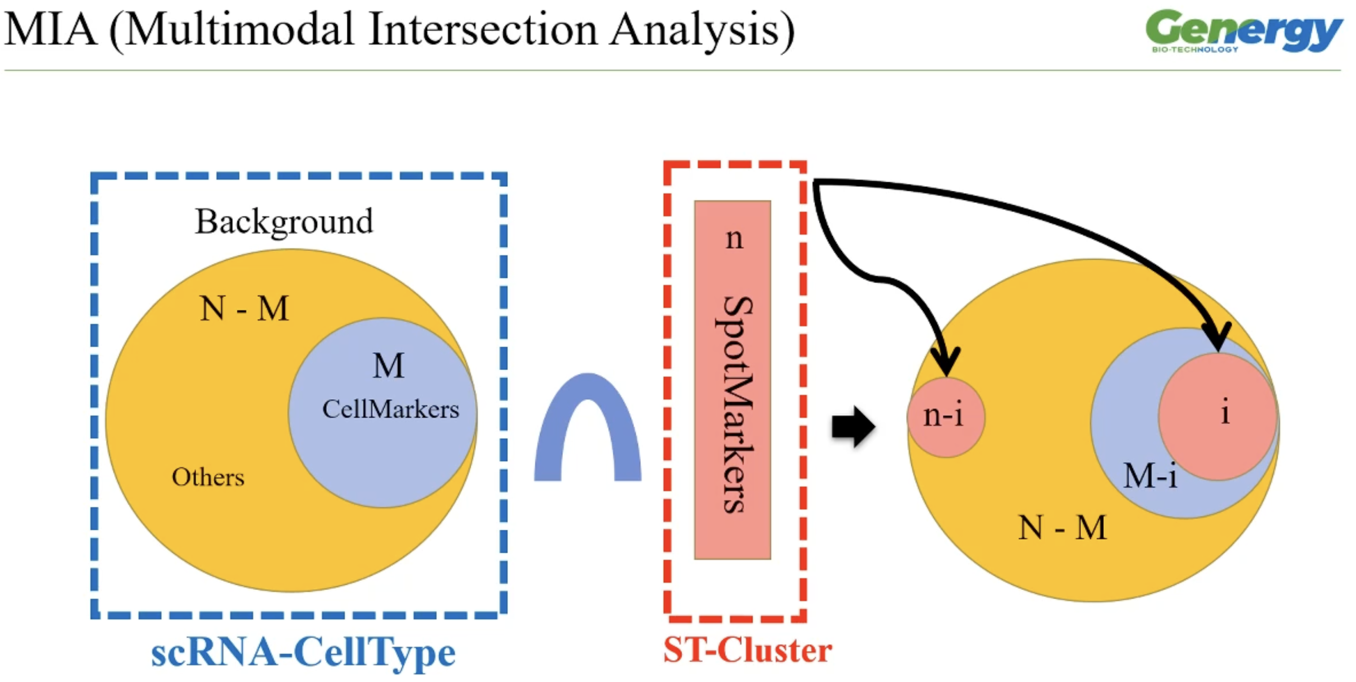
MIA的方法示例图:图片来自晶能生物的公开课

但是其文中,没有给出具体的实现方法,只是简述了原理. 一度让我放弃这个分析方法. 我尝试复现了这个算法的结果,结果非常符合预期.

根据晶能公开课讲师何飞的介绍，利用R中base函数租中的phyper功能就可以实现， 自己根据公式， 写了一个函数来实现MIA的分析目的，但是结果和《NBT》的文章的数据在数量级就不对，我根据MIA的算法，做了更改，结果就变得非常漂亮。非常符合预期。

所以将MIA包装成函数，防在Spat包中，功能取名为MIA_analysis,简单用法如下：

d = MIA_analysis(sc_object = stereo_smn, sp_object = stereo, sc_diff = sc_diff, sp_diff = sp_diff)

输出结果为单细胞数据和空间组数据的关联性判断P值的-log10（即越大，P值越显著）。 其中sc_object和sc_diff分别是scRNA的seurat对象和seurat差异分析的结果矩阵。

注意：差异矩阵必须是每个群与其他所有依次做差异的结果。其实就是默认参数的比较方式。

而sp_diff和sp_object，就是空间组的seurat的对象和差异分析矩阵。

赶紧来尝试下吧！

wangjiaxuan666/Spat documentation built on Jan. 4, 2023, 8:35 a.m.