README.md
In yixuanh/PXStools:
PXStools
PXStools is a R software package to provide tools for conducting exposure association studies. The accompanying paper can be found at:
Installation
The package can be directly downloaded from R:
install.packages("devtools")
The development version from GitHub can be downloaded with:
devtools::install_github("yixuanh/PXStools")
Functions
The package contains five functions:
xwas :conduct an exposure-wide association study (XWAS) across given exposure for a single phenotype. Please refer to https://doi.org/10.1371/journal.pone.0010746 for more details.
plot_coeff_xwas : plots the beta coefficients from the XWAS results.
manhattan_xwas : plots the p values from the XWAS results on a -log scale. Be careful fof any associations that have a p value of close to zero as that will approach infinity in the -log scale.
PXS : conducts the LASSO-based selection procedure on a set of given exposures to build a poly-exposure risk score for a single phenotype. It is recommended that the inputed exposures for PXS are the signficant associations from the XWAS to minimize sample loss.
PXSgl : conducts group LASSO-based procedure on a set of given exposures to build a poly-exposure risk score for a single phenotype. It is recommended that the inputed exposures for PXSgl are the signficant associations from the XWAS to minimize sample loss.
delta_pred : calculates the change in predictive power between two models, e.g. one with and without PXS. For linear mdoels, a change in R2 wil be reported; for logistic regression models, a change in AUC will be reported; for Cox regresison modelx, a change in C index will be reported.
conducts group LASSO-based procedure on a set of given exposures to build a poly-exposure risk score for a single phenotype. It is recommended that the inputed exposures for PXSgl are the signficant associations from the XWAS to minimize sample loss.
Options
In xwas, PXS, and PXSgl functions, the user can input any set of exposures of interest. It is also possible to run different types of regression analysis including lm for linear models, logistic for binary phenotypes, and cox for cox regression. The user can choose a set of covariates (cov) to adjust for at each stage of the analysis as well as which exposure factors to remove (removes) from the analysis. In PXS, the type of regularization (LASSO, elastic net, or ridge regression) can be specificied with alph parameter. Additional documentation for function parameters are described below.
Requirements
The input data frame must have the following columns:
ID: ID of individuals in dataframe
PHENO: phenotype of interest (binary (0/1) or continuous)
if running survival analysis, it must also have
TIME: time to event or censoring
In addition to the the final prediction group, two other groups are needed to train the model.
Parameter Descriptions
xwas(): conducts exposure wide univariate associations between the phenotype of interest and a set of exposures.
df the data frame input
X column name of exposure variables to run XWAS
cov column name of covariates
mod type of model to run; 'lm' for linear regression, 'logistic' for logistic regression; 'cox' for Cox regression
IDA list of IDs to include in XWAS
removes any exposure response, categorical or numerical, to remove from XWAS. This should be in the form of a list
adjust method for adjusting for multiple comparison, see ?p.adjust to see other options
intermdiate saves an intermediate file containing the coefficients of covariates. Default is False
manhattan_xwas(): plots the p values of the XWAS results, analogous to a GWAS manhattan plot. Note: since the y axis is in the -log scale, there may be issues with plotting if the p value is zero or very close to zero (taking the neg log of it will be infinite)
xdff matrix returned from XWAS function, row names of matrix should be the X variables
pval column name of p value
thresh p value threshold for significance
angle rotation of x axis labels. please refer to ggplot2 manual for more detailed description
va vertical adjustment of x axis labels. please refer to ggplot2 manual for more detailed description
ha horizontal adjustment of x axis labels. please refer to ggplot2 manual for more detailed description
size text size of x axis labels. please refer to ggplot2 manual for more detailed description
plot_coeff_xwas(): plots the coefficients of XWAS results
xdff matrix returned from XWAS function, rownames of matrix should be the X variables
pval column name of p value
coeff column name of coefficients
thresh p value threshold for signficance
all default is to plot only signficant associaitons, all=TRUE plots all associatons
PXS(): builds a polyexposure risk score
df the data frame input
X column name of significant exposure variables from XWAS
cov column name of covariates
mod type of model to run; 'lm' for linear regression, 'logistic' for logistic regression; 'cox' for Cox regression
IDA list of IDs to from XWAS procedure
IDB list of IDs for testing set
IDC list of IDs in the final prediction set
seed setting a seed
removes any exposure response, categorical or numerical, to remove from the analysis. This should be in the form of a list
fdr whether or not to adjust for multiple hypothesis correction
intermediate whether or not to save intermediate files
folds number of folds for glmnet cross validation, default is 10
alph the alpha value used in glmnet, alpha = 1 is assumed by default (lasso), setting alpha = 0 for ridge, and anything in between 0 and 1 for elastic net. please refer to glmnet documentation for more details
PXSgl(): builds a polyexposure risk score with consideration of pairwise interactions between exposures using the group lasso method
df the data frame input
X column name of significant exposure variables from XWAS
cov column name of covariates
mod type of model to run; 'lm' for linear regression, 'logistic' for logistic regression; 'cox' for Cox regression
IDA list of IDs to from XWAS procedure
IDB list of IDs for testing set
IDC list of IDs in the final prediction set
seed setting a seed
removes any exposure response, categorical or numerical, to remove from the analysis This should be in the form of a list
fdr whether or not to adjust for multiple hypothesis correction
intermediate whether or not to save intermediate files
folds number of folds for the cross validation step, default is 10
delta_pred(): calculates the change in predictive ability between two models. For linear models, a change in R2 wil be reported; for logistic regression models, a change in AUC will be reported; for Cox regresison models, a change in C index will be reported. The column name of the Y variable must be "PHENO". For Cox regression models, the time to event column name must be "TIME".
df the data frame input
xvarsA column name of variables to include in first model
xvarsB column name of variables to include in second model
mod type of model to run; 'lm' for linear regression, 'logistic' for logistic regression; 'cox' for Cox regression
boot number of bootstrap samples, default is 100
Example (Continuous Phenotype)
This will be an example using the CONT_DF.RData dataset provided in the package. The CONT_DF dataset contains the individual ID, sex, gender, continuous and categorical variables, and a continuous phenotype. We will use SEX, AGE, COV_Q_OTHER, and COV_C_OTHER, as our covariate. The initial set of exposures that we are interested in are VAR_1 through VAR_33. We will be using a linear model.
Store variable names:
set.seed(7)

COV=colnames(CONT_DF)[2:5] #covariate names
XVAR=colnames(CONT_DF)[16:48] #exposure names
REM='L' #remove the response 'L' from our analysis

#randomly sort data into three equal sized group, group C will contain individuals with a final predicted PXS
ss <- sample(1:3,size=nrow(CONT_DF),replace=TRUE,prob=c(1/5,1/5,3/5))
id_A<-CONT_DF$ID[ss==1]
id_B<-CONT_DF$ID[ss==2]
id_C<-CONT_DF$ID[ss==3]
Run XWAS:
XWAS_results=xwas(df=CONT_DF,X=XVAR,cov = COV,mod = 'lm',IDA = id_A,removes = REM)
head(XWAS_results)
#       Estimate Std..Error   t.value     Pr...t.. nrow.stored.          fdr
#VAR_1 494.19110   24.95760 19.801225 1.376340e-73          982 7.384411e-71
#VAR_2 265.40248   32.29990  8.216821 6.619720e-16          982 3.382520e-14
#VAR_3  74.70753   34.29551  2.178347 2.961965e-02          982 9.414615e-01
#VAR_4  77.64219   34.79878  2.231175 2.589671e-02          982 8.683898e-01
#VAR_5  35.98990   34.30748  1.049039 2.944205e-01          982 1.000000e+00
#VAR_6 475.00995   25.62860 18.534368 6.504983e-66          982 2.326725e-63

#obtain significant X's
sigx=row.names(XWAS_results)[which(XWAS_results$fdr<0.05)]
sigx[11:length(sigx)]=substr(sigx[11:length(sigx)],1,nchar(sigx[11:length(sigx)])-1) #remove levels and only keep name of variable
sigx=unique(sigx)

sigx
#[1] "VAR_1"   "VAR_2"   "VAR_6"   "VAR_8"   "VAR_9"   "VAR_10"  "VAR_14"  "VAR_16"  "VAR_17"  "VAR_18"  "VAR_22"  "VAR_25"
Visualize results from XWAS:
manhattan_xwas(xdff = XWAS_results,pval = 'fdr',thresh = 0.05) #plots p values on -log10 scale
plot_coeff_xwas(xdff = XWAS_results,pval = 'fdr',coeff='Estimate',thresh = 0.05) #plots coefficients of significant results, set all=TRUE to plot all results
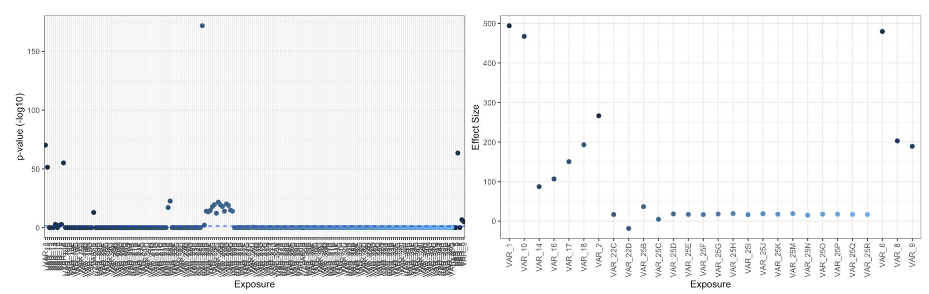
Run PXS (with only signficant exposures):
PXSS=PXS(df=CONT_DF,X=sigx,cov=COV,removes = REM,mod = 'lm',IDA = id_A,IDB = id_B,IDC = id_C,seed=5)

# "intiating PXS procedure with 13 variables"
# "excluding individuals..."
# "914 individuals remain"
# "transformed responsetab"
# "LASSO step initiating..."
# "cross validated LASSO complete"
# "the  min lamda  is: 0.0181050587125221"
# "11 variables remain after LASSO"
# "excluding individuals..."
# "930 individuals remain"
# "8 remain after FS iteration 1"
# 8 remain after final FS iteration, they are:  VAR_22 VAR_25 VAR_1 VAR_2 VAR_6 VAR_8 VAR_10 VAR_17
# "0 individuals removed due to factor having a new level"

nrow(PXSS) #number of individuals with PXS
# 2831

head(PXSS)
#    ID    SEX AGE COV_Q_OTHER COV_C_OTHER        VAR_1         VAR_2        VAR_6         VAR_8      VAR_10       VAR_17 VAR_22 VAR_25 PHENO       PXS
# 4572 FEMALE  47    7.738711  CATEGORY_5  0.003945463 -0.0007426558 -0.009524965 -0.0007623313 -0.02206128 -0.028053092      C      B    95 115.48074
# 2754   MALE  44   15.349081  CATEGORY_5 -0.005833392 -0.0070134080  0.018185588 -0.0192416176 -0.04251531  0.004848575      D      C    77  82.13151
# 2678   MALE  45   15.081943  CATEGORY_4 -0.004395898 -0.0047589039  0.009265629 -0.0152872580  0.00294643  0.018504878      C      B    95 116.52842
# 3064   MALE  50    5.657369  CATEGORY_3 -0.001120768  0.0061214494 -0.007926178  0.0099030477  0.03748063  0.012897271      E      B   116 112.84812
# 3976   MALE  66    1.470289  CATEGORY_2  0.012189827  0.0047791377  0.003133365  0.0117178749 -0.01354368 -0.017855771      G      C   102  93.11601
# 4364 FEMALE  48   16.530377  CATEGORY_1 -0.036801092 -0.0207197737 -0.011525390  0.0050126760 -0.01347574 -0.001232650      D      C    79  77.92055
Get the change in R2 between a model with just baseline covariates versus with the addition of PXS
varsA=COV
varsB=c(COV,'PXS')
delta_pred(PXSS,varsA,varsB,'lm')
# change in R2: 0.835 (0.821, 0.845)
# first model R2:  0.001 (0.001, 0.007)
# second model R2:  0.836 (0.824, 0.846)
````

If you would like to consider interactions in calculate PXS, please use the PXSgl function instead:
```R
PXSinter=PXSgl(df=CONT_DF,X=sigx,cov=COV,removes = REM,mod = 'lm',IDA = id_A,IDB = id_B,IDC = id_C,seed=5)

# "intiating group lasso PXS procedure with 14 variables"
# "excluding individuals..."
# "878 individuals remain"
# "cross validation with 10 folds"
# "the  min lamda  is: 0.00561177934844416"
# "recalibrating model in group B..."
# "excluding individuals..."
# "3614 individuals remain"

nrow(PXSinter) #number of individuals with PXS
# 2727

head(PXSinter)
#    ID    SEX AGE COV_Q_OTHER COV_C_OTHER      PC_1      PC_2       PC_3      PC_4        VAR_1         VAR_2        VAR_6         VAR_8
# 4572 FEMALE  47    7.738711  CATEGORY_5 1.2674114 0.9203929  2.6974477 0.9914804  0.003945463 -0.0007426558 -0.009524965 -0.0007623313
# 2754   MALE  44   15.349081  CATEGORY_5 0.5550317 0.9852589 -2.4922787 2.0085929 -0.005833392 -0.0070134080  0.018185588 -0.0192416176
# 2678   MALE  45   15.081943  CATEGORY_4 0.5632954 1.1129693 -1.5017750 2.6902221 -0.004395898 -0.0047589039  0.009265629 -0.0152872580
# 3064   MALE  50    5.657369  CATEGORY_3 0.1701464 0.9345670  0.5661696 1.1395434 -0.001120768  0.0061214494 -0.007926178  0.0099030477
# 3976   MALE  66    1.470289  CATEGORY_2 1.1001742 0.4358340  0.8061108 1.1374945  0.012189827  0.0047791377  0.003133365  0.0117178749
# 4364 FEMALE  48   16.530377  CATEGORY_1 0.9128850 1.3486736  0.5913076 0.3542070 -0.036801092 -0.0207197737 -0.011525390  0.0050126760
#        VAR_9      VAR_10       VAR_14       VAR_16       VAR_18 VAR_22 VAR_25 VAR_27 PHENO      pred
#  0.014674896 -0.02206128  0.028193331 -0.003030358 -0.021275163      C      B      J    95 117.08439
#  0.010574598 -0.04251531 -0.004591859 -0.021717874  0.026210946      D      C      P    77  90.66943
# -0.037871902  0.00294643 -0.073432151 -0.015424781  0.006503829      C      B      Q    95 125.55657
# -0.001291723  0.03748063  0.002486285  0.009385328 -0.036010278      E      B      Y   116 119.09216
#  0.018172056 -0.01354368  0.030513644 -0.002688886  0.010949063      G      C      U   102 100.76497
# -0.010092473 -0.01347574 -0.010005814 -0.007991927 -0.031461808      D      C      Q    79  77.73137
Example (Binary Phenotype)
This will be an example using the BINARY_DF.RData dataset provided in the package. The BINARY_DF dataset contains the individual ID, sex, gender, continuous and categorical variables, a binary phenotype, and time to event data. We will use SEX, AGE, COV_Q_OTHER, and COV_C_OTHER, as our covariate. The initial set of exposures that we are interested in are VAR_1 through VAR_33. We will be using the logistic model.
set.seed(7)
COV=colnames(BINARY_DF)[2:9] #covariate names
XVAR=colnames(BINARY_DF)[16:50] #exposure names
REM='L' #remove the response 'B' from our analysis

#randomly sort data into three equal sized group, group C will contain individuals with a final predicted PXS
ss <- sample(1:3,size=nrow(BINARY_DF),replace=TRUE,prob=c(1/5,1/5,3/5))
id_A<-BINARY_DF$ID[ss==1]
id_B<-BINARY_DF$ID[ss==2]
id_C<-BINARY_DF$ID[ss==3]
Run XWAS:
XWAS_results=xwas(df=BINARY_DF,X=XVAR,cov = COV,mod = 'logistic',IDA = id_A,removes = REM)
head(XWAS_results)
#        Estimate Std..Error    z.value     Pr...z.. nrow.stored.          fdr
#VAR_1 66.8837233   5.362552 12.4723671 1.056406e-35          982 1.307498e-32
#VAR_2 24.7163927   4.629661  5.3387043 9.361316e-08          982 1.655195e-05
#VAR_3  5.7229386   4.568069  1.2528136 2.102736e-01          982 1.000000e+00
#VAR_4 10.7767723   4.657384  2.3139112 2.067259e-02          982 8.822817e-01
#VAR_5 -0.8885037   4.547791 -0.1953704 8.451030e-01          982 1.000000e+00
#VAR_6 64.0887303   5.296899 12.0992930 1.065247e-33          982 6.592203e-31

#obtain significant X's
sigx=row.names(XWAS_results)[which(XWAS_results$fdr<0.05)]
sigx[8:length(sigx)]=substr(sigx[8:length(sigx)],1,nchar(sigx[8:length(sigx)])-1) #remove levels and only keep name of variable
sigx=unique(sigx)

sigx
# "VAR_1"   "VAR_2"   "VAR_6"   "VAR_8"   "VAR_9"   "VAR_10"  "VAR_18"  "VAR_22"  "VAR_25"
Visualize results from XWAS:
manhattan_xwas(xdff = XWAS_results,pval = 'fdr',thresh = 0.05) #plots p values on -log10 scale
plot_coeff_xwas(xdff = XWAS_results,pval = 'fdr',coeff='Estimate',thresh = 0.05) #plots coefficients of significant results, set all=TRUE to plot all results
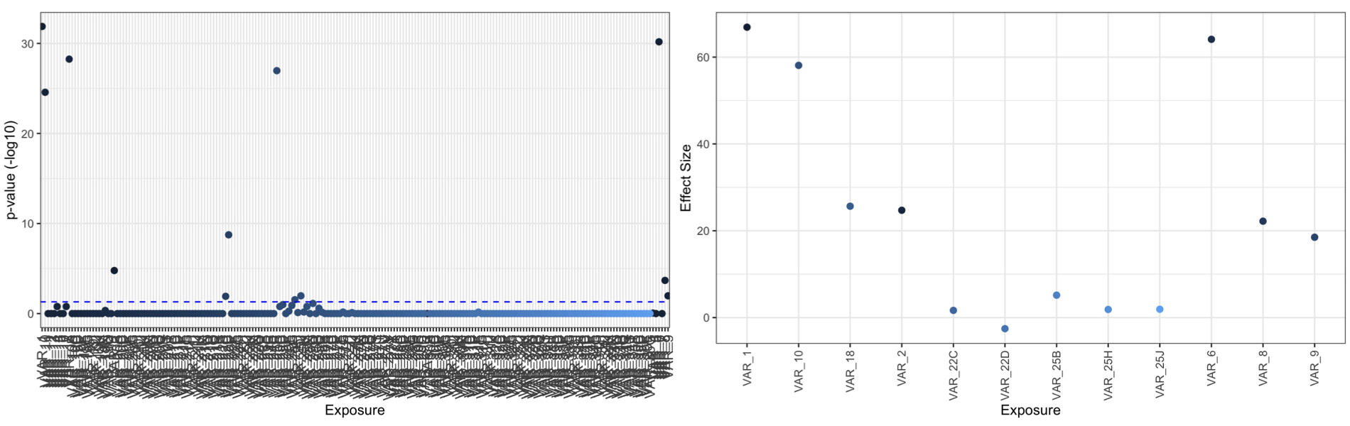
Run PXS (with only signficant exposures):
#PXSS=PXS(df=BINARY_DF,X=sigx,cov=COV,removes = REM,mod = 'logistic',IDA = id_A,IDB = id_B,IDC = id_C,seed=5)
#intiating PXS procedure with 9 variables
#excluding individuals...
#914 individuals remain
#transformed responsetab
#LASSO initiating...
#cross validation complete
#the  min lamda  is: 0.0313078739623684
#9 variables remain after regularization
#excluding individuals...
#930 individuals remain
#5 remain after BackS iteration 1
#5 remain after final BackS iteration, they are:  VAR_22 VAR_25 VAR_1 VAR_6 VAR_8
#0 individuals removed due to factor having a new level
By default, PXS uses LASSO regularization. Elastic net or ridge regression can also be implemented by specifying the alpha value. As an example, we can rerun PXS with ridge regression:
PXSS=PXS(df=BINARY_DF,X=sigx,cov=COV,removes = REM,mod = 'logistic',IDA = id_A,IDB = id_B,IDC = id_C,seed=5,alph=0)
#intiating PXS procedure with 10 variables
#excluding individuals...
#914 individuals remain
#transformed responsetab
#ridge regression initiating...
#cross validation complete
#the  min lamda  is: 0.0313078739623684
#9 variables remain after regularization
#excluding individuals...
#930 individuals remain
#5 remain after BackS iteration 1
#5 remain after final BackS iteration, they are:  VAR_22 VAR_25 VAR_1 VAR_6 VAR_8
#0 individuals removed due to factor having a new level
To get the change in AUC between a model with just baseline covariates versus with the addition of PXS:
varsA=COV
varsB=c(COV,'PXS')
delta_pred(PXSS,varsA,varsB,'logistic')
# change in AUC: 0.377 (0.338, 0.385)
# first model AUC: 0.526 (0.527, 0.563)
# second model AUC: 0.903 (0.892, 0.914)
````

## Example (Survival Analysis)
This will be an example using the ``BINARY_DF.RData`` dataset provided in the package. The BINARY_DF dataset contains the individual ID, sex, gender, continuous and categorical variables, a binary phenotype, and time to event data. We will use SEX, AGE, COV_Q_OTHER, and COV_C_OTHER, as our covariate. The initial set of exposures that we are interested in are VAR_1 through VAR_33. We will be using the logistic model.

```R
set.seed(7)
load('/Users/yixuanhe/Dropbox (HMS)/PATEL/R_Packages/PXStools/PXStools/data/BINARY_DF.RData')
COV=colnames(BINARY_DF)[2:9] #covariate names
XVAR=colnames(BINARY_DF)[16:50] #exposure names
REM='L' #remove the response 'B' from our analysis

#randomly sort data into three equal sized group, group C will contain individuals with a final predicted PXS
ss <- sample(1:3,size=nrow(BINARY_DF),replace=TRUE,prob=c(1/5,1/5,3/5))
id_A<-BINARY_DF$ID[ss==1]
id_B<-BINARY_DF$ID[ss==2]
id_C<-BINARY_DF$ID[ss==3]
Run XWAS
XWAS_results=xwas(df=BINARY_DF,X=XVAR,cov = COV,mod = 'cox',IDA = id_A,removes = REM)
head(XWAS_results)

#           coef    exp.coef. se.coef.          z     Pr...z.. nrow.stored.          fdr
#VAR_1 27.877006 1.278880e+12 2.669075 10.4444442 1.553628e-25          982 1.922903e-22
#VAR_2  8.728393 6.175793e+03 2.853299  3.0590533 2.220377e-03          982 2.217052e-01
#VAR_3  5.004221 1.490409e+02 3.054618  1.6382478 1.013700e-01          982 1.000000e+00
#VAR_4 10.088868 2.407353e+04 3.079373  3.2762737 1.051866e-03          982 1.446532e-01
#VAR_5  1.307285 3.696126e+00 3.061649  0.4269873 6.693886e-01          982 1.000000e+00
#VAR_6 27.202800 6.516670e+11 2.730609  9.9621720 2.231337e-23          982 9.205645e-21

#obtain significant X's
sigx=row.names(XWAS_results)[which(XWAS_results$fdr<0.05)]
sigx[5:length(sigx)]=substr(sigx[5:length(sigx)],1,nchar(sigx[5:length(sigx)])-1) #remove levels and only keep name of variable
sigx=unique(sigx)

sigx
#"VAR_1"  "VAR_6"  "VAR_10" "VAR_18" "VAR_22" "VAR_25"
Visualize results from XWAS:
manhattan_xwas(xdff = XWAS_results,pval = 'fdr',thresh = 0.05) #plots p values on -log10 scale
plot_coeff_xwas(xdff = XWAS_results,pval = 'fdr',coeff='coef',thresh = 0.05) #plots coefficients of significant results, set all=TRUE to plot all results
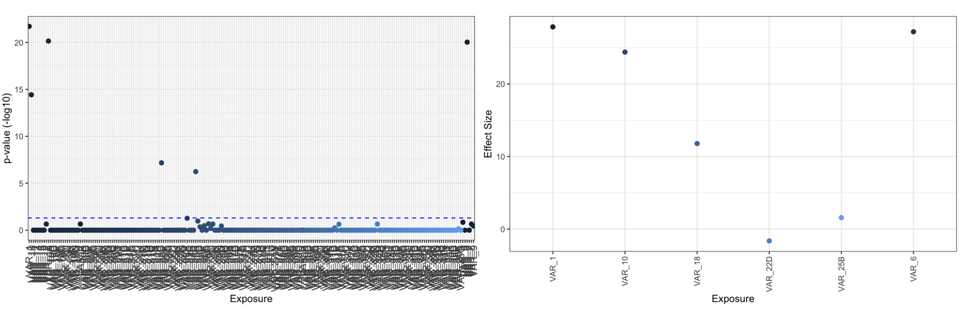
Build PXS:
PXSS=PXS(df=BINARY_DF,X=sigx,cov=COV,removes = REM,mod = 'cox',IDA = id_A,IDB = id_B,IDC = id_C,seed=5)
#intiating PXS procedure with 6 variables
#excluding individuals...
#914 individuals remain
#transformed responsetab
#LASSO initiating...
#cross validated LASSO complete
#the  min lamda  is: 0.026512783464246
#5 variables remain after LASSO
#excluding individuals...
#930 individuals remain
#4 remain after BackS iteration 1
#4 remain after final BackS iteration, they are:  VAR_25 VAR_1 VAR_10 VAR_18
#0 individuals removed due to factor having a new level
To get the change in C index between a model with just baseline covariates versus with the addition of PXS:
```R
varsA=COV
varsB=c(COV,'PXS')
delta_pred(PXSS,varsA,varsB,'lm')
change in C index: 0.148 (0.123, 0.162)
first model C index: 0.522 (0.512, 0.547)
second model C index: 0.67 (0.658, 0.683)
````
To note: for survival anlysis, delta_pred() is only able to get change in C index. If you would like to get the net reclassification index (NRI), please check out existing methods such as the 'nricens' R package.
yixuanh/PXStools documentation built on July 27, 2022, 10:27 a.m.
R Package Documentation
Browse R Packages
We want your feedback!
Note that we can't provide technical support on individual packages. You should contact the package authors for that.
PXStools
PXStools is a R software package to provide tools for conducting exposure association studies. The accompanying paper can be found at:
Installation
The package can be directly downloaded from R:
install.packages("devtools")
The development version from GitHub can be downloaded with:
devtools::install_github("yixuanh/PXStools")
Functions
The package contains five functions:
xwas :conduct an exposure-wide association study (XWAS) across given exposure for a single phenotype. Please refer to https://doi.org/10.1371/journal.pone.0010746 for more details.
plot_coeff_xwas : plots the beta coefficients from the XWAS results.
manhattan_xwas : plots the p values from the XWAS results on a -log scale. Be careful fof any associations that have a p value of close to zero as that will approach infinity in the -log scale.
PXS : conducts the LASSO-based selection procedure on a set of given exposures to build a poly-exposure risk score for a single phenotype. It is recommended that the inputed exposures for PXS are the signficant associations from the XWAS to minimize sample loss.
PXSgl : conducts group LASSO-based procedure on a set of given exposures to build a poly-exposure risk score for a single phenotype. It is recommended that the inputed exposures for PXSgl are the signficant associations from the XWAS to minimize sample loss.
delta_pred : calculates the change in predictive power between two models, e.g. one with and without PXS. For linear mdoels, a change in R2 wil be reported; for logistic regression models, a change in AUC will be reported; for Cox regresison modelx, a change in C index will be reported.
conducts group LASSO-based procedure on a set of given exposures to build a poly-exposure risk score for a single phenotype. It is recommended that the inputed exposures for PXSgl are the signficant associations from the XWAS to minimize sample loss.
Options
In xwas, PXS, and PXSgl functions, the user can input any set of exposures of interest. It is also possible to run different types of regression analysis including lm for linear models, logistic for binary phenotypes, and cox for cox regression. The user can choose a set of covariates (cov) to adjust for at each stage of the analysis as well as which exposure factors to remove (removes) from the analysis. In PXS, the type of regularization (LASSO, elastic net, or ridge regression) can be specificied with alph parameter. Additional documentation for function parameters are described below.
Requirements
The input data frame must have the following columns:
ID: ID of individuals in dataframe
PHENO: phenotype of interest (binary (0/1) or continuous)
if running survival analysis, it must also have
TIME: time to event or censoring
In addition to the the final prediction group, two other groups are needed to train the model.
Parameter Descriptions
xwas(): conducts exposure wide univariate associations between the phenotype of interest and a set of exposures.
df the data frame input
X column name of exposure variables to run XWAS
cov column name of covariates
mod type of model to run; 'lm' for linear regression, 'logistic' for logistic regression; 'cox' for Cox regression
IDA list of IDs to include in XWAS
removes any exposure response, categorical or numerical, to remove from XWAS. This should be in the form of a list
adjust method for adjusting for multiple comparison, see ?p.adjust to see other options
intermdiate saves an intermediate file containing the coefficients of covariates. Default is False
manhattan_xwas(): plots the p values of the XWAS results, analogous to a GWAS manhattan plot. Note: since the y axis is in the -log scale, there may be issues with plotting if the p value is zero or very close to zero (taking the neg log of it will be infinite)
xdff matrix returned from XWAS function, row names of matrix should be the X variables
pval column name of p value
thresh p value threshold for significance
angle rotation of x axis labels. please refer to ggplot2 manual for more detailed description
va vertical adjustment of x axis labels. please refer to ggplot2 manual for more detailed description
ha horizontal adjustment of x axis labels. please refer to ggplot2 manual for more detailed description
size text size of x axis labels. please refer to ggplot2 manual for more detailed description
plot_coeff_xwas(): plots the coefficients of XWAS results
xdff matrix returned from XWAS function, rownames of matrix should be the X variables
pval column name of p value
coeff column name of coefficients
thresh p value threshold for signficance
all default is to plot only signficant associaitons, all=TRUE plots all associatons
PXS(): builds a polyexposure risk score
df the data frame input
X column name of significant exposure variables from XWAS
cov column name of covariates
mod type of model to run; 'lm' for linear regression, 'logistic' for logistic regression; 'cox' for Cox regression
IDA list of IDs to from XWAS procedure
IDB list of IDs for testing set
IDC list of IDs in the final prediction set
seed setting a seed
removes any exposure response, categorical or numerical, to remove from the analysis. This should be in the form of a list
fdr whether or not to adjust for multiple hypothesis correction
intermediate whether or not to save intermediate files
folds number of folds for glmnet cross validation, default is 10
alph the alpha value used in glmnet, alpha = 1 is assumed by default (lasso), setting alpha = 0 for ridge, and anything in between 0 and 1 for elastic net. please refer to glmnet documentation for more details
PXSgl(): builds a polyexposure risk score with consideration of pairwise interactions between exposures using the group lasso method
df the data frame input
X column name of significant exposure variables from XWAS
cov column name of covariates
mod type of model to run; 'lm' for linear regression, 'logistic' for logistic regression; 'cox' for Cox regression
IDA list of IDs to from XWAS procedure
IDB list of IDs for testing set
IDC list of IDs in the final prediction set
seed setting a seed
removes any exposure response, categorical or numerical, to remove from the analysis This should be in the form of a list
fdr whether or not to adjust for multiple hypothesis correction
intermediate whether or not to save intermediate files
folds number of folds for the cross validation step, default is 10
delta_pred(): calculates the change in predictive ability between two models. For linear models, a change in R2 wil be reported; for logistic regression models, a change in AUC will be reported; for Cox regresison models, a change in C index will be reported. The column name of the Y variable must be "PHENO". For Cox regression models, the time to event column name must be "TIME".
df the data frame input
xvarsA column name of variables to include in first model
xvarsB column name of variables to include in second model
mod type of model to run; 'lm' for linear regression, 'logistic' for logistic regression; 'cox' for Cox regression
boot number of bootstrap samples, default is 100
Example (Continuous Phenotype)
This will be an example using the CONT_DF.RData dataset provided in the package. The CONT_DF dataset contains the individual ID, sex, gender, continuous and categorical variables, and a continuous phenotype. We will use SEX, AGE, COV_Q_OTHER, and COV_C_OTHER, as our covariate. The initial set of exposures that we are interested in are VAR_1 through VAR_33. We will be using a linear model.
Store variable names:
set.seed(7)
COV=colnames(CONT_DF)[2:5] #covariate names
XVAR=colnames(CONT_DF)[16:48] #exposure names
REM='L' #remove the response 'L' from our analysis
#randomly sort data into three equal sized group, group C will contain individuals with a final predicted PXS
ss <- sample(1:3,size=nrow(CONT_DF),replace=TRUE,prob=c(1/5,1/5,3/5))
id_A<-CONT_DF$ID[ss==1]
id_B<-CONT_DF$ID[ss==2]
id_C<-CONT_DF$ID[ss==3]
Run XWAS:
XWAS_results=xwas(df=CONT_DF,X=XVAR,cov = COV,mod = 'lm',IDA = id_A,removes = REM)
head(XWAS_results)
# Estimate Std..Error t.value Pr...t.. nrow.stored. fdr
#VAR_1 494.19110 24.95760 19.801225 1.376340e-73 982 7.384411e-71
#VAR_2 265.40248 32.29990 8.216821 6.619720e-16 982 3.382520e-14
#VAR_3 74.70753 34.29551 2.178347 2.961965e-02 982 9.414615e-01
#VAR_4 77.64219 34.79878 2.231175 2.589671e-02 982 8.683898e-01
#VAR_5 35.98990 34.30748 1.049039 2.944205e-01 982 1.000000e+00
#VAR_6 475.00995 25.62860 18.534368 6.504983e-66 982 2.326725e-63
#obtain significant X's
sigx=row.names(XWAS_results)[which(XWAS_results$fdr<0.05)]
sigx[11:length(sigx)]=substr(sigx[11:length(sigx)],1,nchar(sigx[11:length(sigx)])-1) #remove levels and only keep name of variable
sigx=unique(sigx)
sigx
#[1] "VAR_1" "VAR_2" "VAR_6" "VAR_8" "VAR_9" "VAR_10" "VAR_14" "VAR_16" "VAR_17" "VAR_18" "VAR_22" "VAR_25"
Visualize results from XWAS:
manhattan_xwas(xdff = XWAS_results,pval = 'fdr',thresh = 0.05) #plots p values on -log10 scale
plot_coeff_xwas(xdff = XWAS_results,pval = 'fdr',coeff='Estimate',thresh = 0.05) #plots coefficients of significant results, set all=TRUE to plot all results
Run PXS (with only signficant exposures):
PXSS=PXS(df=CONT_DF,X=sigx,cov=COV,removes = REM,mod = 'lm',IDA = id_A,IDB = id_B,IDC = id_C,seed=5)
# "intiating PXS procedure with 13 variables"
# "excluding individuals..."
# "914 individuals remain"
# "transformed responsetab"
# "LASSO step initiating..."
# "cross validated LASSO complete"
# "the min lamda is: 0.0181050587125221"
# "11 variables remain after LASSO"
# "excluding individuals..."
# "930 individuals remain"
# "8 remain after FS iteration 1"
# 8 remain after final FS iteration, they are: VAR_22 VAR_25 VAR_1 VAR_2 VAR_6 VAR_8 VAR_10 VAR_17
# "0 individuals removed due to factor having a new level"
nrow(PXSS) #number of individuals with PXS
# 2831
head(PXSS)
# ID SEX AGE COV_Q_OTHER COV_C_OTHER VAR_1 VAR_2 VAR_6 VAR_8 VAR_10 VAR_17 VAR_22 VAR_25 PHENO PXS
# 4572 FEMALE 47 7.738711 CATEGORY_5 0.003945463 -0.0007426558 -0.009524965 -0.0007623313 -0.02206128 -0.028053092 C B 95 115.48074
# 2754 MALE 44 15.349081 CATEGORY_5 -0.005833392 -0.0070134080 0.018185588 -0.0192416176 -0.04251531 0.004848575 D C 77 82.13151
# 2678 MALE 45 15.081943 CATEGORY_4 -0.004395898 -0.0047589039 0.009265629 -0.0152872580 0.00294643 0.018504878 C B 95 116.52842
# 3064 MALE 50 5.657369 CATEGORY_3 -0.001120768 0.0061214494 -0.007926178 0.0099030477 0.03748063 0.012897271 E B 116 112.84812
# 3976 MALE 66 1.470289 CATEGORY_2 0.012189827 0.0047791377 0.003133365 0.0117178749 -0.01354368 -0.017855771 G C 102 93.11601
# 4364 FEMALE 48 16.530377 CATEGORY_1 -0.036801092 -0.0207197737 -0.011525390 0.0050126760 -0.01347574 -0.001232650 D C 79 77.92055
Get the change in R2 between a model with just baseline covariates versus with the addition of PXS
varsA=COV
varsB=c(COV,'PXS')
delta_pred(PXSS,varsA,varsB,'lm')
# change in R2: 0.835 (0.821, 0.845)
# first model R2: 0.001 (0.001, 0.007)
# second model R2: 0.836 (0.824, 0.846)
````
If you would like to consider interactions in calculate PXS, please use the PXSgl function instead:
```R
PXSinter=PXSgl(df=CONT_DF,X=sigx,cov=COV,removes = REM,mod = 'lm',IDA = id_A,IDB = id_B,IDC = id_C,seed=5)
# "intiating group lasso PXS procedure with 14 variables"
# "excluding individuals..."
# "878 individuals remain"
# "cross validation with 10 folds"
# "the min lamda is: 0.00561177934844416"
# "recalibrating model in group B..."
# "excluding individuals..."
# "3614 individuals remain"
nrow(PXSinter) #number of individuals with PXS
# 2727
head(PXSinter)
# ID SEX AGE COV_Q_OTHER COV_C_OTHER PC_1 PC_2 PC_3 PC_4 VAR_1 VAR_2 VAR_6 VAR_8
# 4572 FEMALE 47 7.738711 CATEGORY_5 1.2674114 0.9203929 2.6974477 0.9914804 0.003945463 -0.0007426558 -0.009524965 -0.0007623313
# 2754 MALE 44 15.349081 CATEGORY_5 0.5550317 0.9852589 -2.4922787 2.0085929 -0.005833392 -0.0070134080 0.018185588 -0.0192416176
# 2678 MALE 45 15.081943 CATEGORY_4 0.5632954 1.1129693 -1.5017750 2.6902221 -0.004395898 -0.0047589039 0.009265629 -0.0152872580
# 3064 MALE 50 5.657369 CATEGORY_3 0.1701464 0.9345670 0.5661696 1.1395434 -0.001120768 0.0061214494 -0.007926178 0.0099030477
# 3976 MALE 66 1.470289 CATEGORY_2 1.1001742 0.4358340 0.8061108 1.1374945 0.012189827 0.0047791377 0.003133365 0.0117178749
# 4364 FEMALE 48 16.530377 CATEGORY_1 0.9128850 1.3486736 0.5913076 0.3542070 -0.036801092 -0.0207197737 -0.011525390 0.0050126760
# VAR_9 VAR_10 VAR_14 VAR_16 VAR_18 VAR_22 VAR_25 VAR_27 PHENO pred
# 0.014674896 -0.02206128 0.028193331 -0.003030358 -0.021275163 C B J 95 117.08439
# 0.010574598 -0.04251531 -0.004591859 -0.021717874 0.026210946 D C P 77 90.66943
# -0.037871902 0.00294643 -0.073432151 -0.015424781 0.006503829 C B Q 95 125.55657
# -0.001291723 0.03748063 0.002486285 0.009385328 -0.036010278 E B Y 116 119.09216
# 0.018172056 -0.01354368 0.030513644 -0.002688886 0.010949063 G C U 102 100.76497
# -0.010092473 -0.01347574 -0.010005814 -0.007991927 -0.031461808 D C Q 79 77.73137
Example (Binary Phenotype)
This will be an example using the BINARY_DF.RData dataset provided in the package. The BINARY_DF dataset contains the individual ID, sex, gender, continuous and categorical variables, a binary phenotype, and time to event data. We will use SEX, AGE, COV_Q_OTHER, and COV_C_OTHER, as our covariate. The initial set of exposures that we are interested in are VAR_1 through VAR_33. We will be using the logistic model.
set.seed(7)
COV=colnames(BINARY_DF)[2:9] #covariate names
XVAR=colnames(BINARY_DF)[16:50] #exposure names
REM='L' #remove the response 'B' from our analysis
#randomly sort data into three equal sized group, group C will contain individuals with a final predicted PXS
ss <- sample(1:3,size=nrow(BINARY_DF),replace=TRUE,prob=c(1/5,1/5,3/5))
id_A<-BINARY_DF$ID[ss==1]
id_B<-BINARY_DF$ID[ss==2]
id_C<-BINARY_DF$ID[ss==3]
Run XWAS:
XWAS_results=xwas(df=BINARY_DF,X=XVAR,cov = COV,mod = 'logistic',IDA = id_A,removes = REM)
head(XWAS_results)
# Estimate Std..Error z.value Pr...z.. nrow.stored. fdr
#VAR_1 66.8837233 5.362552 12.4723671 1.056406e-35 982 1.307498e-32
#VAR_2 24.7163927 4.629661 5.3387043 9.361316e-08 982 1.655195e-05
#VAR_3 5.7229386 4.568069 1.2528136 2.102736e-01 982 1.000000e+00
#VAR_4 10.7767723 4.657384 2.3139112 2.067259e-02 982 8.822817e-01
#VAR_5 -0.8885037 4.547791 -0.1953704 8.451030e-01 982 1.000000e+00
#VAR_6 64.0887303 5.296899 12.0992930 1.065247e-33 982 6.592203e-31
#obtain significant X's
sigx=row.names(XWAS_results)[which(XWAS_results$fdr<0.05)]
sigx[8:length(sigx)]=substr(sigx[8:length(sigx)],1,nchar(sigx[8:length(sigx)])-1) #remove levels and only keep name of variable
sigx=unique(sigx)
sigx
# "VAR_1" "VAR_2" "VAR_6" "VAR_8" "VAR_9" "VAR_10" "VAR_18" "VAR_22" "VAR_25"
Visualize results from XWAS:
manhattan_xwas(xdff = XWAS_results,pval = 'fdr',thresh = 0.05) #plots p values on -log10 scale
plot_coeff_xwas(xdff = XWAS_results,pval = 'fdr',coeff='Estimate',thresh = 0.05) #plots coefficients of significant results, set all=TRUE to plot all results
Run PXS (with only signficant exposures):
#PXSS=PXS(df=BINARY_DF,X=sigx,cov=COV,removes = REM,mod = 'logistic',IDA = id_A,IDB = id_B,IDC = id_C,seed=5)
#intiating PXS procedure with 9 variables
#excluding individuals...
#914 individuals remain
#transformed responsetab
#LASSO initiating...
#cross validation complete
#the min lamda is: 0.0313078739623684
#9 variables remain after regularization
#excluding individuals...
#930 individuals remain
#5 remain after BackS iteration 1
#5 remain after final BackS iteration, they are: VAR_22 VAR_25 VAR_1 VAR_6 VAR_8
#0 individuals removed due to factor having a new level
By default, PXS uses LASSO regularization. Elastic net or ridge regression can also be implemented by specifying the alpha value. As an example, we can rerun PXS with ridge regression:
PXSS=PXS(df=BINARY_DF,X=sigx,cov=COV,removes = REM,mod = 'logistic',IDA = id_A,IDB = id_B,IDC = id_C,seed=5,alph=0)
#intiating PXS procedure with 10 variables
#excluding individuals...
#914 individuals remain
#transformed responsetab
#ridge regression initiating...
#cross validation complete
#the min lamda is: 0.0313078739623684
#9 variables remain after regularization
#excluding individuals...
#930 individuals remain
#5 remain after BackS iteration 1
#5 remain after final BackS iteration, they are: VAR_22 VAR_25 VAR_1 VAR_6 VAR_8
#0 individuals removed due to factor having a new level
To get the change in AUC between a model with just baseline covariates versus with the addition of PXS:
varsA=COV
varsB=c(COV,'PXS')
delta_pred(PXSS,varsA,varsB,'logistic')
# change in AUC: 0.377 (0.338, 0.385)
# first model AUC: 0.526 (0.527, 0.563)
# second model AUC: 0.903 (0.892, 0.914)
````
## Example (Survival Analysis)
This will be an example using the ``BINARY_DF.RData`` dataset provided in the package. The BINARY_DF dataset contains the individual ID, sex, gender, continuous and categorical variables, a binary phenotype, and time to event data. We will use SEX, AGE, COV_Q_OTHER, and COV_C_OTHER, as our covariate. The initial set of exposures that we are interested in are VAR_1 through VAR_33. We will be using the logistic model.
```R
set.seed(7)
load('/Users/yixuanhe/Dropbox (HMS)/PATEL/R_Packages/PXStools/PXStools/data/BINARY_DF.RData')
COV=colnames(BINARY_DF)[2:9] #covariate names
XVAR=colnames(BINARY_DF)[16:50] #exposure names
REM='L' #remove the response 'B' from our analysis
#randomly sort data into three equal sized group, group C will contain individuals with a final predicted PXS
ss <- sample(1:3,size=nrow(BINARY_DF),replace=TRUE,prob=c(1/5,1/5,3/5))
id_A<-BINARY_DF$ID[ss==1]
id_B<-BINARY_DF$ID[ss==2]
id_C<-BINARY_DF$ID[ss==3]
Run XWAS
XWAS_results=xwas(df=BINARY_DF,X=XVAR,cov = COV,mod = 'cox',IDA = id_A,removes = REM)
head(XWAS_results)
# coef exp.coef. se.coef. z Pr...z.. nrow.stored. fdr
#VAR_1 27.877006 1.278880e+12 2.669075 10.4444442 1.553628e-25 982 1.922903e-22
#VAR_2 8.728393 6.175793e+03 2.853299 3.0590533 2.220377e-03 982 2.217052e-01
#VAR_3 5.004221 1.490409e+02 3.054618 1.6382478 1.013700e-01 982 1.000000e+00
#VAR_4 10.088868 2.407353e+04 3.079373 3.2762737 1.051866e-03 982 1.446532e-01
#VAR_5 1.307285 3.696126e+00 3.061649 0.4269873 6.693886e-01 982 1.000000e+00
#VAR_6 27.202800 6.516670e+11 2.730609 9.9621720 2.231337e-23 982 9.205645e-21
#obtain significant X's
sigx=row.names(XWAS_results)[which(XWAS_results$fdr<0.05)]
sigx[5:length(sigx)]=substr(sigx[5:length(sigx)],1,nchar(sigx[5:length(sigx)])-1) #remove levels and only keep name of variable
sigx=unique(sigx)
sigx
#"VAR_1" "VAR_6" "VAR_10" "VAR_18" "VAR_22" "VAR_25"
Visualize results from XWAS:
manhattan_xwas(xdff = XWAS_results,pval = 'fdr',thresh = 0.05) #plots p values on -log10 scale
plot_coeff_xwas(xdff = XWAS_results,pval = 'fdr',coeff='coef',thresh = 0.05) #plots coefficients of significant results, set all=TRUE to plot all results
Build PXS:
PXSS=PXS(df=BINARY_DF,X=sigx,cov=COV,removes = REM,mod = 'cox',IDA = id_A,IDB = id_B,IDC = id_C,seed=5)
#intiating PXS procedure with 6 variables
#excluding individuals...
#914 individuals remain
#transformed responsetab
#LASSO initiating...
#cross validated LASSO complete
#the min lamda is: 0.026512783464246
#5 variables remain after LASSO
#excluding individuals...
#930 individuals remain
#4 remain after BackS iteration 1
#4 remain after final BackS iteration, they are: VAR_25 VAR_1 VAR_10 VAR_18
#0 individuals removed due to factor having a new level
To get the change in C index between a model with just baseline covariates versus with the addition of PXS:
```R varsA=COV varsB=c(COV,'PXS') delta_pred(PXSS,varsA,varsB,'lm')
change in C index: 0.148 (0.123, 0.162)
first model C index: 0.522 (0.512, 0.547)
second model C index: 0.67 (0.658, 0.683)
```` To note: for survival anlysis, delta_pred() is only able to get change in C index. If you would like to get the net reclassification index (NRI), please check out existing methods such as the 'nricens' R package.
R Package Documentation
Browse R Packages
We want your feedback!
Note that we can't provide technical support on individual packages. You should contact the package authors for that.
Embedding an R snippet on your website
Add the following code to your website.
For more information on customizing the embed code, read Embedding Snippets.