MetAlyzer User Guide
In MetAlyzer: Read and Analyze 'MetIDQ™' Software Output Files

knitr::opts_chunk$set(echo=TRUE, cache=TRUE, collapse=T, comment='#>')
library(MetAlyzer)
library(SummarizedExperiment)
library(ggplot2)
library(dplyr)

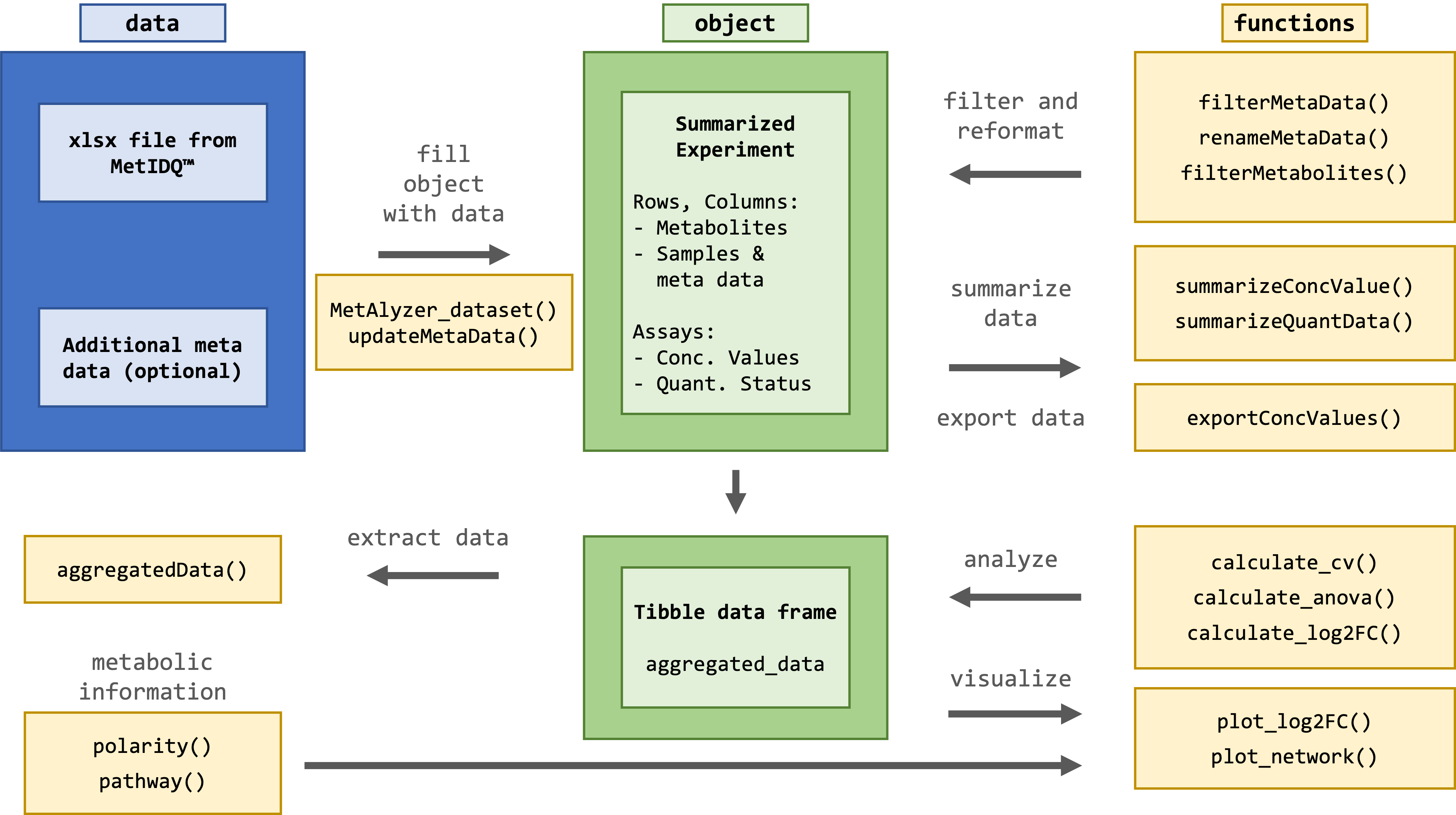
::: {style="text-align: justify"} The package provides methods to read output files from the MetIDQ™ software into R. Metabolomics data is read and reformatted into an S4 object for convenient data handling, statistics and downstream analysis. :::

Install

There is a version available on CRAN.

install.packages("MetAlyzer")

The latest version can directly be installed from the github.

library(devtools)
install_github("nilsmechtel/MetAlyzer")

Overview

{width="100%"}

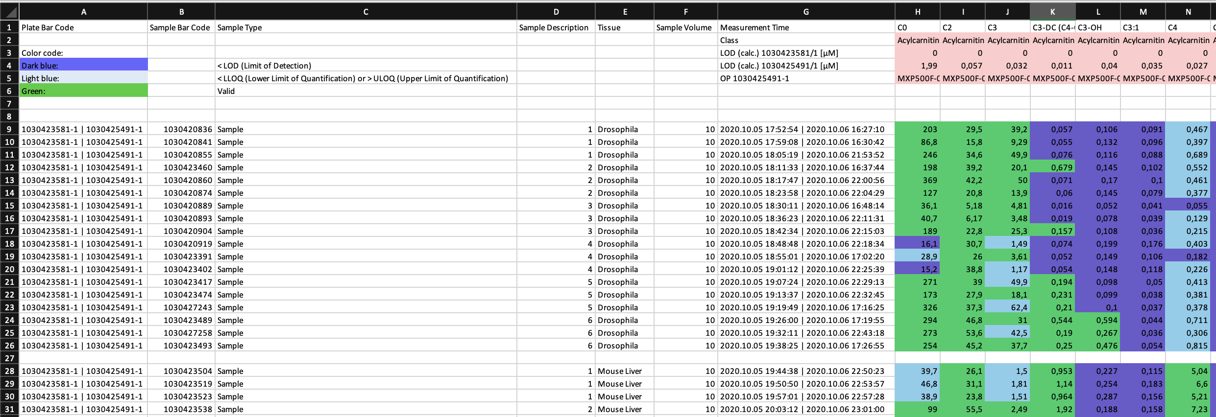
::: {style="text-align: justify"} The package takes metabolomic measurements as ".xlsx" files generated from the MetIDQ™ software. Additionally, meta data for each sample can be provided for further analysis. :::

::: {style="text-align: justify"} Effective quantification of metabolites requires a reliable signal. The limit of detection (LOD) is defined as 3 times signal-to-noise of the baseline, calculated by the software MetIDQ™ for each metabolite. Values are classified as "Valid", "LOQ" (below limit of quantification) or "LOD" (below limit of detection). This information is encoded in the color in the ".xlsx" table. Further color codes can include "ISTD Out of Range", "Invalid" and "Incomplete". The MetAlyzer packages allow to read both information, the value and the quantification status, gives statistics about the quantification efficacy and allows filtering based on the LOD. :::

Example of excel sheet. {width="100%"}

Get started

::: {style="text-align: justify"} To present the base functionalities of MetAlyzer, we use a data set published by Gegner et al. 2022. This data set was analyzed using the MxP®Quant 500 kit and inlcudes 6 different extraction methods (1 to 6) to quantify 630 metabolites in triplicates for 4 tissue types (Drosophila, Mouse Liver, Mouse Kidney, Zebrafish Liver). It is included in the MetAlyzer package and can be accessed via example_extraction_data(). MetAlyzer_dataset reads the data from Excel into R and stores it as a SummarizedExperiment (SE). :::

fpath <- example_extraction_data()
metalyzer_se <- MetAlyzer_dataset(file_path = fpath)

metalyzer_se

::: {style="text-align: justify"} The SE includes assay information with concentration values and quantification status, while storing metabolites and their respective classes in the row data. It is important to note that there are 630 metabolites, and 232 metabolite indicators calculated using the MetIDQ™ software. Sample-wise metadata is stored in the column data. Additional data such as the file path ('file_path'), the Excel sheet number ('sheet_index'), a list of colors for each quantification status (status_list), as well as a tibble of aggregated concentration data and quantification status for downstream analysis and visualizations ('aggregated_data') are stored in the SE's metadata. :::

::: {style="text-align: justify"} Summaries of concentration values and quantification status are automatically called during data loading, but can also manually be called using summarizeConcValues(metalyzer_se) and summarizeQuantData(metalyzer_se). The function summarizeConcValues prints the quantiles and the amount / percentage of NAs in the concentration data. The function summarizeQuantData gives an overview of the quantification status of the metabolites. E.g 34.16% of metabolites where below the Limit of Detection.

The various elements within the SummarizedExperiment (SE) can be accessed in a manner consistent with a typical SE. :::

meta_data <- colData(metalyzer_se)
head(meta_data)

metabolites <- rowData(metalyzer_se)
head(metabolites)

concentration_values <- assays(metalyzer_se)$conc_values
head(concentration_values, c(5, 5))

quantification_status <- assays(metalyzer_se)$quant_status
head(quantification_status, c(5, 5))

::: {style="text-align: justify"} In addition to accessing the aggregated data through metadata(metalyzer_se)$aggregated_data, it can be directly accessed using aggregatedData. :::

aggregated_data <- aggregatedData(metalyzer_se)
head(aggregated_data)

Manage metabolites and sample-wise meta data

::: {style="text-align: justify"} The functions filterMetabolites and filterMetaData can be used to subset the data set based on certain metabolites or meta variables. Both functions subset conc_values, quant_status and aggregated_data. :::

::: {style="text-align: justify"} Individual metabolites as well as metabolic classes can be passed to filterMetabolites. Here, we want to exclude the metabolism indicators. :::

metalyzer_se <- filterMetabolites(metalyzer_se, drop_metabolites = "Metabolism Indicators")
metalyzer_se

::: {style="text-align: justify"} The extraction methods are encoded in the column "Sample Description" of the meta data. There are 2 blank samples in the data that we want to remove and only keep extraction method 1 to 6. :::

metalyzer_se <- filterMetaData(metalyzer_se, `Sample Description` %in% 1:6)

::: {style="text-align: justify"} To be more specific and for easier handling, we change the column "Sample Description" of the meta data to "Extraction_Method". :::

metalyzer_se <- renameMetaData(metalyzer_se, "Extraction_Method" = "Sample Description")

meta_data <- colData(metalyzer_se)
head(meta_data)

::: {style="text-align: justify"} Additional meta data can be easily added to the Summarized Experiment. Here, we want to add the column "Date" with the current date to the meta data as well as the column "Replicate" with extraction method replicates. :::

replicate_meta_data <- example_meta_data()
head(replicate_meta_data)

metalyzer_se <- updateMetaData(
  metalyzer_se,
  Date = Sys.Date(),
  Replicate = replicate_meta_data$Replicate
)

meta_data <- colData(metalyzer_se)
head(meta_data)

Analysis of extraction methods

::: {style="text-align: justify"} MetAlyzer includes functions to perform data analysis as it was performed for MetaboExtract (Andresen et al. 2022). All analysing functions in MetAlyzer use the aggregated concentration data and quantification status ('aggregated_data'). The calculate_cv calculates the mean, standard deviation (SD) and the coefficient of variation (CV) within each group and saves it to 'aggregated_data'. Each group is additionally categorized into given thresholds of variation based on the calculated CV. :::

metalyzer_se <- calculate_cv(
  metalyzer_se,
  groups = c("Tissue", "Extraction_Method", "Metabolite"),
  cv_thresholds = c(0.1, 0.2, 0.3),
  na.rm = TRUE
)

aggregated_data <- aggregatedData(metalyzer_se) %>%
  select(c(Extraction_Method, Metabolite, Mean, SD, CV, CV_thresh))
head(aggregated_data)

::: {style="text-align: justify"} As described in Gegner et al., an ANOVA is calculated to identify extraction methods with superior and inferior extraction performance. NAs or zero values are first imputed, to avoid NAs during log2 transformation. To impute NAs, the impute_NA argument can be set to TRUE. The argument impute_perc_of_min specifies the percentage of the minimum concentration value that is used for imputation. :::

metalyzer_se <- calculate_anova(
  metalyzer_se,
  categorical = "Extraction_Method",
  groups = c("Tissue", "Metabolite"),
  impute_perc_of_min = 0.2,
  impute_NA = TRUE
)

aggregated_data <- aggregatedData(metalyzer_se) %>%
  select(c(Extraction_Method, Metabolite, imputed_Conc, log2_Conc, ANOVA_n, ANOVA_Group))
head(aggregated_data)

::: {style="text-align: justify"} The result of the imputation is stored in an extra column "imputed_Conc". In total 12,212 zero values were imputed in this example. :::

cat("Number of zero values before imputation:",
    sum(aggregatedData(metalyzer_se)$Concentration == 0, na.rm = TRUE), "\n")

cat("Number of zero values after imputation:",
    sum(aggregatedData(metalyzer_se)$imputed_Conc == 0, na.rm = TRUE), "\n")

Analysis and visualization of treatment data

::: {style="text-align: justify"} MetAlyzer also includes functions to calculate and visualize the log2 fold change of data with paired effects. For this, we load a dataset with control and mutated samples analyzed using the MxP®Quant 500 XL kit. The XL kit covers 332 additional metabolites and 6 additional metabolic classes compared to the MxP®Quant 500 kit. :::

fpath <- example_mutation_data_xl()
metalyzer_se <- MetAlyzer_dataset(file_path = fpath)

metalyzer_se

::: {style="text-align: justify"} Again, we want to remove the metabolism indicators. :::

metalyzer_se <- filterMetabolites(metalyzer_se, drop_metabolites = "Metabolism Indicators")
metalyzer_se

::: {style="text-align: justify"} In this data set, the column "Sample Description" holds information about the wether a sample is a wild type or a mutant. :::

meta_data <- colData(metalyzer_se)
meta_data$`Sample Description`

::: {style="text-align: justify"} To determine the direction of the effect during log2 fold change calculation, the information is converted into a factor and saved as a new column "Control_Mutant". The log2 fold change will now be calculated from "Control" to "Mutant". :::

control_mutant <- factor(colData(metalyzer_se)$`Sample Description`, levels = c("Control", "Mutant"))
metalyzer_se <- updateMetaData(metalyzer_se, Control_Mutant = control_mutant)

meta_data <- colData(metalyzer_se)
meta_data$Control_Mutant

::: {style="text-align: justify"} In order to avoid NAs during log2 transformation the same imputation of NAs or zero values is applied as for calculate_anova. To impute NAs, the impute_NA argument can be set to TRUE. The argument impute_perc_of_min specifies the percentage of the minimum concentration value that is used for imputation. :::

metalyzer_se <- calculate_log2FC(
  metalyzer_se,
  categorical = "Control_Mutant",
  impute_perc_of_min = 0.2,
  impute_NA = TRUE
)

::: {style="text-align: justify"} In addition to accessing the log2 fold change data through metadata(metalyzer_se)$log2FC, it can be directly accessed using log2FC. :::

log2FC(metalyzer_se)

::: {style="text-align: justify"} The log2 fold change between the wild type and the mutant can be visualized with a volcano plot: :::

log2fc_vulcano <- plot_log2FC(
  metalyzer_se,
  hide_labels_for = rownames(rowData(metalyzer_se)),
  vulcano=TRUE
)

log2fc_vulcano

::: {style="text-align: justify"} as well as in a scatter plot categorized by metabolic classes: :::

log2fc_by_class <- plot_log2FC(
  metalyzer_se,
  hide_labels_for = rownames(rowData(metalyzer_se)),
  vulcano=FALSE
)

log2fc_by_class

::: {style="text-align: justify"} MetAlyzer also provides a visualization of the log2 fold change across different pathways, in order to identify groups of metabolites impacted by the effect. :::

log2fc_network <- plot_network(
  metalyzer_se,
  q_value=0.05,
  metabolite_text_size=2,
  connection_width=0.75,
  pathway_text_size=4,
  pathway_width=4,
  scale_colors = c("green", "black", "magenta")
)

log2fc_network