|

In metagear: Comprehensive Research Synthesis Tools for Systematic Reviews and Meta-Analysis

---

title: |

Basic examples of screening studies, extracting data and meta-analysis with the metagear package for R

author: 'Marc J. Lajeunesse' date: University of South Florida, February 12th 2021 (vignette v. 0.7 for metagear v. 0.7)

output: word_document: toc: yes html_document: smart: no toc: yes pdf_document: keep_tex: yes latex_engine: xelatex toc: yes

---

options(width = 800)

Introduction

---

The metagear package for R contains tools for facilitating systematic reviews, data extraction, and meta-analyses. It aims to facilitate research synthesis as a whole, by providing a single source for several of the common tasks involved in screening studies, extracting outcomes from studies, and performing statistical analyses on these outcomes using meta-analysis. Below are a few illustrative examples of applications of these functionalities.

Updates to these examples will be posted on our research webpage at USF, and for previous vignette versions see v. 0.4, v. 0.3, v. 0.2 and v. 0.1.

For the source code of metagear see: http://cran.r-project.org/web/packages/metagear/index.html.

Acknowledgements

Funding for metagear is supported by National Science Foundation (NSF) grants DBI-1262545 and DEB-1451031.

I also thank J. Richardson, J. Zydek, N. Ogburn, B. MacNeill, J. Zloty, and my colleagues in the OpenMEE software team, J. Gurevitch and B. Wallace, for persuading me to develop tools in R.

How to cite?

Lajeunesse, M.J. (2016) Facilitating systematic reviews, data extraction and meta-analysis with the *metagear* package for *R*. *Methods in Ecology and Evolution* **7**: 323-330. [article link](http://onlinelibrary.wiley.com/doi/10.1111/2041-210X.12472/abstract)

Installation and Dependencies

Metagear has several external dependencies that need to be installed and loaded prior to use in R. The first is the EBImage R package (Pau et al. 2010) available only from Bioconductor repository.

To properly install metagear, use the following script in R:

# first load Bioconductor resources needed to install the EBImage package 
# and accept/download all of its dependencies
install.packages("BiocManager"); 
BiocManager::install("EBImage")

# then load metagear
library(metagear)

Finally for Mac OS users, installation is sometimes not straighforward, as the abstract_screener() requires the Tcl/Tk GUI toolkit to be installed. You can get this toolkit by making sure that the latest X11 application (xQuartz) is installed from here: xquartz.macosforge.org.

Report a bug? Have comments or suggestions?

Please email me any bugs, comments, or suggestions and I'll try to include them in future releases: [e-mail]. Also try to include metagear in the subject heading of your email. Finally, I'm open to almost anything, but expect a lag before I respond and/or new additions are added.

Delegating reference screening effort to a team

---

One of the first tasks of a systematic review is to screen the titles and abstracts of study references to assess their relevance for the synthesis project. For example, after a bibliographic search using Web of Science, there may be thousands of references generated; references from experimental studies, modeling studies, review papers, commentaries, etc. These need to be reviewed individually as a first pass to exclude those that do not fit the synthesis project; such as excluding simulation studies that do not report experimental outcomes useful for estimating an effect size.

However, individually screening thousands of references is time consuming, and large synthesis projects may benefit from delegating this screening effort to a research team. Having multiple people screen references also provides an opportunity to assess the repeatability of these screening decisions.

In this example, we have the following goals:

1. Initialize a dataframe containing bibliographic data (tile, abstract, journal) from multiple study references.
2. Distribute these references randomly to two team members.
3. Merge and summarize the screening efforts of this team.

First, let's start by loading and exploring the contents of a pre-packaged dataset from metagear that contains the bibliographic information of 11 journal articles (example_references_metagear). These data are a subset of references generated from a search in Web of Science for "Genome size", and contain the abstracts, titles, volume, page numbers, and authors of these references.

# load package
library(metagear)
# load a bibliographic dataset with the authors, titles, and abstracts of multiple study references 
data(example_references_metagear)
# display the bibliographic variables in this dataset
names(example_references_metagear)
# display the various Journals that these references were published in
example_references_metagear["JOURNAL"]

Our next step is to initialize/prime this dataset for screening tasks. Our goal is to distribute screening efforts to two screeners/reviewers: "Christina" and "Luc". Here each reviewer will screen a separate subset of these references (a forthcoming example will review how to set up a dual screening design where each member screens the same references). The dataset first needs to be initialized as follows:

# prime the study-reference dataset
theRefs <- effort_initialize(example_references_metagear)
# display the new columns added by effort_initialize 
names(theRefs)

Note that the effort_initialize() function added three new columns: "STUDY_ID" which is a unique number for each reference (e.g., from 1 to 11), "REVIEWERS" an empty column with NAs that will be later populated with our reviewers (e.g., Christina and Luc), and finally the "INCLUDE" column, which will later contain the screening efforts by the two reviewers.

Screening efforts are essentially how individual study references get coded for inclusion in the synthesis project; currently the "INCLUDE" column has each reference coded as "not vetted", indicating that each reference has yet to be screened.

Our next task is to delegate screening efforts to our two reviewers Christina and Luc. Our goal is to randomly distribute these references to each reviewer.

# randomly distribute screening effort to a team
theTeam <- c("Christina", "Luc")
theRefs_unscreened <- effort_distribute(theRefs, reviewers = theTeam)
# display screening tasks
theRefs_unscreened[c("STUDY_ID", "REVIEWERS")]

The screening efforts can also be delegated unevenly, such as below where Luc will take on 80% of the screening effort:

# randomly distribute screening effort to a team, but with Luc handeling 80% of the work
theRefs_unscreened <- effort_distribute(theRefs, reviewers = theTeam, effort = c(20, 80))
theRefs_unscreened[c("STUDY_ID", "REVIEWERS")]

The effort can also be redistributed with the effort_redistribute() function. In the above example we assigned Luc 80% of the work. Now let's redistribute half of Luc's work to a new team member "Patsy".

theRefs_Patsy <- effort_redistribute(theRefs_unscreened, 
                                     reviewer = "Luc",
                                     remove_effort = 50, # move 50% of Luc's work to Patsy
                                     reviewers = c("Luc", "Patsy")) # team members loosing and picking up work
theRefs_Patsy[c("STUDY_ID", "REVIEWERS")]

The references have now been randomly assigned to either Christina or Luc. The whole initialization of the reference dataset with effort_initialize() can be abbreviated with effort_distribute(example_references_metagear, reviewers = c("Christina", "Luc"), initialize = TRUE).

Now that screening tasks have been distributed, the next stage is for reviewers to start the manual screening of each assigned reference. This is perhaps best done by providing a separate file of these references to Christina and Luc. They can then work on screening these references separately and remotely. Once the screening is complete, we can then merge these files into a complete dataset (we'll get to this later).

The effort_distribute() function can also save to file each reference subset; these can be given to Christina and Luc to start their work. This is done by setting the 'save_split' parameter to TRUE.

# randomly distribute screening effort to a team, but with Luc handling 80% of the work, 
# but also saving these screening tasks to separate files for each team member
theRefs_unscreened <- effort_distribute(theRefs, reviewers = theTeam, effort = c(20, 80), save_split = TRUE)
theRefs_unscreened[c("STUDY_ID", "REVIEWERS")]
list.files(pattern = "effort")

These two effort_*.csv files contain the assigned references for Christina and Luc. These can be passed on to each team member so that they can begin screening/coding each reference for inclusion in the synthesis project.

References should be coded as "YES" or "NO" for inclusion, but can also be coded as "MAYBE" if bibliographic information is missing or there is inadequate information to make a proper assessment of the study.

The abstract_screener() function can be used to facilitate this screening process (an example is forthcoming), but for the sake of introducing how screening efforts can be merged and summarized, I manually coded all the references in both of Christina's and Luc's effort_*.csv files. Essentially, I randomly coded each references as either "YES", "NO", or "MAYBE". These files now contain the completed screening efforts.

We can merge these two files with the completed screening efforts using the effort_merge() function, as well as summarize the outcome of screening tasks using the effort_summary() function.

# HIDDEN: randomly populate the INCLUDE columns of effort_Luc.csv and effort_Christina.csv with
# random inclusion codes of YES, NO, MAYBE
lapply(list.files(getwd(), pattern = "effort"), 
       function(x) {
        tempCSV <- read.csv(x, header = TRUE)
        tempCSV["INCLUDE"] <- sample(c("YES","NO","MAYBE"), nrow(tempCSV), replace = TRUE)
        write.csv(tempCSV, x)
        return(tempCSV)
       }
      )

# merge the effort_Luc.csv and effort_Christina.csv 
# WARNING: will merge all files named "effort_*" in directory
theRefs_screened <- effort_merge()
theRefs_screened[c("STUDY_ID", "REVIEWERS", "INCLUDE")]
theSummary <- effort_summary(theRefs_screened)

# HIDDEN: clean up generated files
file.remove("effort_Christina.csv")
file.remove("effort_Luc.csv")

The summary of screening tasks describes the outcomes of which references had studies appropriate for the synthesis project, while also outlining which need to be re-assessed. The team should discuss these challenging references and decide if they are appropriate for inclusion or track down any additional/missing information needed to make proper assessment of their inclusion.

Screening abstracts of references

---

Metagear offers a simple abstract screener to quickly sift through the abstracts and titles of multiple references. Here is some script to help initialize the screener GUI in R:

# load package
library(metagear)

# initialize bibliographic data and screening tasks
data(example_references_metagear)
effort_distribute(example_references_metagear, initialize = TRUE, reviewers = "marc", save_split = TRUE)

# initialize screener GUI
abstract_screener("effort_marc.csv", aReviewer = "marc")

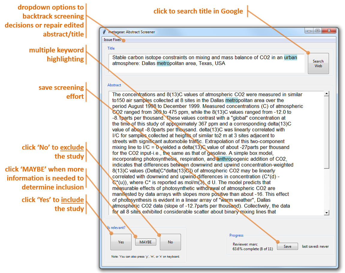
The GUI itself will appear as a single window with the first title/abstract listed in the .csv file. If abstracts have already been screened/coded, it will begin at the nearest reference labeled as "not vetted". The SEARCH WEB button opens the default browser and searches Google with the title of the reference. The YES, MAYBE, NO buttons, which also have shortcuts ALT-Y and ALT-N, are used to code the inclusion/exclusion of the reference. Once clicked/coded the next reference is loaded. The SAVE button is used to save the coding progress of screening tasks. It will save coding progress directly to the loaded .csv file. Closing the GUI and not saving will result in the loss of screening efforts relative to last save.

Here's what to expect with this GUI (note that depending on the platform running R, the layout of this GUI will differ slightly):

Workflow example

---

Here I provide a quick example of extracting effect size data from a journal article PDF.

In this example, we have the following goals:

1. Get the DOI from a study reference.
2. Use this DOI to download a PDF of the journal article.
3. Extract all the figures from this PDF.
4. And finally, extract the effect size from one of these figures.

First, let's start by using one of the DOIs from the pre-packaged metagear dataset that contains the bibliographic information of 11 journal articles (example_references_metagear). These data are a subset of references generated from a search in Web of Science for "Genome size", and contain the abstracts, titles, volume, page numbers, and authors of these references.

# load package
library(metagear)
# load a bibliographic dataset with the DOIs
data(example_references_metagear)
# display one of the DOI's reference
theBiblio <- scrape_bibliography(example_references_metagear$DOI[4])
theBiblio$citation

Our next goal is to download a PDF of the Ruas et al.'s (2008) journal article and then extract its figures.

# locate and download a PDF of this journal article
PDF_download(example_references_metagear$DOI[4], theFileName = "Ruas_2008")

A PDF was found, successfully downloaded, and saved as "Ruas_2008.pdf". Next let's extract the figures from this PDF and select the one with potential effect size data. Here we will extract and save the figures as image files (jpegs), and then plot each one to see which is a regression figure.

# extract figures from the PDF
imageFiles <- PDF_extractImages("Ruas_2008.pdf")

# plot all figures with file names
par(mfrow=c(2,3), las = 1)
for(i in 1:6) {
  figure_display(imageFiles[i])
  mtext(imageFiles[i], col = "red", cex = 1.2)
}

It seems like the file "Ruas_2008_bin_4.jpg" is a regression plot; let's try to extract the effect size (correlation coefficient) from this regression.

# plot the regression figure
figure_display("Ruas_2008_bin_4.jpg")
# extract the correlation coefficient
rawData <- figure_scatterPlot("Ruas_2008_bin_4.jpg")

Well... regression points were detected using the default settings of figure_scatterPlot, but so were many more objects. Let's change the settings to detect diamond points rather than circles, and let's also increase the point size since the figure image is large.

# plot the regression figure
rawData <- figure_scatterPlot("Ruas_2008_bin_4.jpg", 
                              point_shape = "diamond", # circle shapes to diamonds
                              point_size = 5) # increase from 3 to 5 in size

The regression point detection was much more successful here, and although some detections were flagged as potential errors, every point in the figure was detected. Further, the estimated regression coefficients were very similar to those reported within the figure. To get better coefficients it is necessary to explicitly define the scale of each axis scale as follows (however note that the correlation coefficient will not change):

# plot the regression figure
rawData <- figure_scatterPlot("Ruas_2008_bin_4.jpg", 
                              point_shape = "diamond", # circle shapes to diamonds
                              point_size = 5, # increase from 3 to 5 in size
                              X_min = 0.12,
                              X_max = 0.52,
                              Y_min = 1.8,
                              Y_max = 7.2)

# HIDDEN: clean up downloaded PDF and all extracted image files
theList <- list.files(pattern = "Ruas_2008")
lapply(theList, file.remove)

The estimated coefficients are not as reported; perhaps they are reversed in the figure or there are data points not present in the figure and these are found outside the visual range of each axis.

Downloading PDFs

---

Once references have been screened, metagear can be used to download and organize the full-texts of these references. However, note that the download success of these PDFs is entirely conditional on the journal subscription coverage of the host institution running metagear. Also note that metagear only supports the download of a PDF article if the DOI (digital object identifier) is available for that article.

In this example, we have the following goals:

1. Download a single PDF with the PDF_download() function.
2. Download multiple PDFs with the PDFs_collect() function.

Let's start by loading the pre-packaged reference dataset in metagear that contains the bibliographic information of 11 journal articles (example_references_metagear). This dataset includes a column "DOI" which contains the DOI of each article (if available).

# load package
library(metagear)
# load a bibliographic dataset with the DOIs
data(example_references_metagear)
# display the year published of each study reference and their DOIs
example_references_metagear[c("JOURNAL", "DOI")]

Note that references collected from bibliographic databases like Web of Science will often be incomplete. For example, the study published in EVOLUTIONARY ECOLOGY RESEARCH does not have a DOI (described above as NA). This is because EVOLUTIONARY ECOLOGY RESEARCH is an independently published journal and does not provide DOIs for their research articles.

However, a DOI for the AMERICAN NATURALIST study is available, and let's use it to fetch the PDF.

# load package
PDF_download("10.1086/319928", theFileName = "AMNAT_metagear")

# HIDDEN: clean up generated files
lapply(c("AMNAT_metagear.pdf"), file.remove)

The downloader provides information on the download success, and in this case a PDF was successfully retrieved. It was saved in the working directory of the R process (to see this directory use getwd()).

Now let's try downloading all the PDFs from our reference dataset. This can be done using the PDFs_collect() function.

# (optional) initialize the reference dataset to help generate standardized fileNames (e.g., STUDY_ID numbers)
theRefs <- effort_initialize(example_references_metagear)
# fetch the PDFs
collectionOutcomes <- PDFs_collect(theRefs, DOIcolumn = "DOI", FileNamecolumn = "STUDY_ID", quiet = TRUE)
table(collectionOutcomes$downloadOutcomes)

# HIDDEN: clean up downloaded files
lapply(c("1.pdf", "3.pdf", "4.pdf", "5.pdf", "6.1.pdf", "6.2.pdf", "8.pdf", "10.pdf", "11.pdf"), file.remove)

Eight of the 11 references had successful PDF downloads; the remaining 3 did not have DOIs available. These PDFs will need to be checked to determine if their contents are the desired research articles. Also note that the downloading process will take time, and in general, it will take ~ 45 seconds to detect and download a single PDF.

Scraping Web of Science for bibliographic data

---

Metagear can also scrape Web of Science (WOS) for bibliographic data if the DOI (digital object identifier) of a study is available. Currently, only the authors, title, publication year, journal, issue, page numbers, number of references, number of citations, and the journal impact factor (and year released) are fetched for a study. By default, scrape_bibliography() will print an MLA-like formatted citation of the article.

For example, let's quickly scrape WOS for Carmona et al.’s (2011) reference and its number of citations.

# load package
library(metagear)
# display the DOI's reference and number of citations
theBiblio <- scrape_bibliography("10.1111/j.1365-2435.2010.01794.x")
# number of citations
print(paste(theBiblio$N_citations, "citations as of", theBiblio$date_scraped))

Generating PRISMA plots

---

PRISMA plots (preferred reporting items for systematic reviews and meta-analyses), or PRISMA flow diagrams, are an important and simple way to present the flow of information on how studies were found, collated, and screened for systematic reviews and meta-analysis (Liberati et al. 2009). Generally, they depict from top to bottom the original number of studies identified through bibliographic databases (and other sources) and how this population of studies was culled for inclusion into the synthesis project.

Metagear offers an easy way to generate PRISMA plots, this requires a list of the 'phases' of the screening process. It also requires certain phases to be labeled to properly depict the start (with the string START_PHASE:) and exclusion (string EXCLUDE_PHASE:) phases of the flow diagram. Below is a quick example.

# load package
library(metagear)

phases <- c("START_PHASE: # of studies identified through database searching",
            "START_PHASE: # of additional studies identified through other sources",
            "# of studies after duplicates removed",
            "# of studies with title and abstract screened",
            "EXCLUDE_PHASE: # of studies excluded",
            "# of full-text articles assessed for eligibility",
            "EXCLUDE_PHASE: # of full-text articles excluded, not fitting eligibility criteria",
            "# of studies included in qualitative synthesis",
            "EXCLUDE_PHASE: # studies excluded, incomplete data reported",
            "final # of studies included in quantitative synthesis (meta-analysis)")
thePlot <- plot_PRISMA(phases)

Generating different PRISMA plot layouts

There are also several different PRISMA plot layouts available to generate simpler or more colourful schemes. Below are a few of the various designs available, and for example, here the cinnamonMint scheme can be generated using: plot_PRISMA(phases, design = "cinnamonMint").

# load package
library(metagear)

phases <- c("START_PHASE: # of studies identified through database searching",
            "START_PHASE: # of additional studies identified through other sources",
            "# of studies after duplicates removed",
            "# of studies with title and abstract screened",
            "EXCLUDE_PHASE: # of studies excluded",
            "# of full-text articles assessed for eligibility",
            "EXCLUDE_PHASE: # of full-text articles excluded, not fitting eligibility criteria",
            "# of studies included in qualitative synthesis",
            "EXCLUDE_PHASE: # studies excluded, incomplete data reported",
            "final # of studies included in quantitative synthesis (meta-analysis)")

# plot various PRISMA design layouts
par(mfrow = c(2, 2), las = 1)
designExamples <- c("cinnamonMint", "grey", "greyMono", "vintage")
for(i in designExamples) {
  theFile <- paste0(i, ".png")
  png(theFile, width = 12, height = 12, units = "in", res = 450)
    plot_PRISMA(phases, design = i)
  dev.off() 
  figure_display(theFile)
  mtext(i, side = 2, line = -2, col = "black", cex = 0.9)
  file.remove(theFile)
}

It is also possible to individually customize various design features of the PRISMA plot. Here are some of the features that can be modified:

| parameter | options | |-----+-------| | S | color of start phases (default: white) | | P | color of the main phases (default: white) | | E | color of the exclusion phases (default: white) | | F | color of the final phase (default: white) | | fontSize | the size of the font (default: 12) | | fontColor | the font color (default: black) | | fontFace | either plain, bold, italic, or bold.italic (default: plain) | | flatArrow | arrows curved when FALSE (default); arrows square when TRUE | | flatBox | boxes curved when FALSE (default); boxes square when TRUE |

Here's a quick example on how to change the color of the exclusion phases:

# load package
library(metagear)

phases <- c("START_PHASE: # of studies identified through database searching",
            "# of studies after duplicates removed",
            "# of studies with title and abstract screened",
            "EXCLUDE_PHASE: # of studies excluded",
            "# of full-text articles assessed for eligibility",
            "EXCLUDE_PHASE: # of full-text articles excluded, not fitting eligibility criteria",
            "# of studies included in qualitative synthesis",
            "EXCLUDE_PHASE: # studies excluded, incomplete data reported",
            "final # of studies included in quantitative synthesis (meta-analysis)")

# PRISMA plot with custom layout
thePlot <- plot_PRISMA(phases, design = c(E = "lightcoral", flatArrow = TRUE))

Notes on PRISMA plotting since metagear v. 0.1 and 0.2

Previous versions of metagear (v. 0.2 and 0.1) offered a more flexible version of plot_PRISMA() that allowed for proper rescaling of PRISMA objects when the user manually changed the window size of the plot. Unfortunately, this version did not load well when bundled with the package and yielded unusual plots (I would love to hear any tips on how to properly manage viewports and grid objects within a package!). Anyway, these versions are available on my website and allow for higher-quality PRISMA plots; these old functions can be downloaded here and work best when not loaded with metagear.

Automated extraction of data from scatterplots

---

Extracting data from a figure image is a common challenge when trying to extract outcomes (effect sizes) from a study. The scrapping (reverse engineering) of data points from a scatterplot image can be automated with metagear.

In these examples, we have the following goals:

1. Extract data points from an image containing a scatterplot using the figure_scatterPlot() default parameters.
2. Tweak the parameters to extract data from scatterplots with various formats (e.g., different point shapes, or image sizes).

Example 1 | figure_scatterPlot() default settings

Metagear offers a pre-packaged scatterplot image, and so let's begin with extracting data from this image, before moving to more advanced applications of figure_scatterPlot(). First, let's load and display the image.

# load metagear package and .jpg image manipulation package EBImage
library(metagear)
library(EBImage)
# load the scatterplot image, source: Kam et al. (2003) Functional Ecology 17:496-503.
Kam_et_al_2003_Fig2 <- system.file("images", "Kam_et_al_2003_Fig2.jpg", package = "metagear")
# display the image
figure_display(Kam_et_al_2003_Fig2) 

Now let's use figure_scatterPlot() to scrape data from this image; however, because Kam_et_al_2003_Fig2 is pre-packaged with metagear it needs to be converted back to a .jpg before the image can be processed.

The figure_scatterPlot() will by default output three objects:

1. The estimated regression fit of these detected points, as well as the estimated effect size and variance of the correlation presented in the figure.
2. A raster image of the detected objects painted over the original image. Blue spheres are detected points, orange spheres are detected clusters of points that could not be separated, the X-axis in pink, and the Y-axis in green. The points and axes can also be extracted individually using the figure_detectAllPoints() and figure_detectAxis() functions.
3. The X and Y data from each detected point on the image, and information on whether that point was identified as a cluster.

Here are the results of using figure_scatterPlot() on Kam et al.'s (2002) figure.

# load the scatterplot image, source: Kam et al. (2003) Functional Ecology 17:496-503.
rawData <- figure_scatterPlot(Kam_et_al_2003_Fig2) 

The estimated regression coefficients are very similar to those originally reported by Kam et al.'s (2002) study; which were Y = 12.03 + 0.907 * X with an R2 = 0.59 and a sample size of N = 51.

Example 2 | tweaking defaults for image size

Now let's try to extract data from another image. This time the figure is relatively small and figure_scatterPlot() will need some adjustments based on this size difference. Also, this time we will scale the data extractions to the X- and Y-axis scale; this is useful to calculate the original regression coefficients. Here, the minimum and maximum presented in the figure for the X-axis is 0 to 50, and 0 to 70 for the Y-axis. However, note that re-scaling the data does not affect the effect size calculated from the figure, only the estimated regression coefficients. Let's download the image first from my website and then process it.

# download the figure image from my website
figureSource <- "http://lajeunesse.myweb.usf.edu/metagear/example_2_scatterPlot.jpg"
download.file(figureSource, "example_2_scatterPlot.jpg", quiet = TRUE, mode = "wb")
aFig <- figure_read("example_2_scatterPlot.jpg", display = TRUE)
# because of the small size of the image the axis parameter needed adjustment from 5 to 3
rawData2 <- figure_scatterPlot("example_2_scatterPlot.jpg",  
                               axis_thickness = 3, # adjusted from 5 to 3 to help detect the thin axis
                               X_min = 0, # minimum X-value reported in the plot
                               X_max = 50, # maximum X-value reported in the plot
                               Y_min = 0,
                               Y_max = 70)

# HIDDEN: clean up downloaded image file
file.remove("example_2_scatterPlot.jpg")

In this example, because of the small size of the figure, the axis_thinkness parameter needed to be reduced from 5 to 3. This was sufficient to detect the axis lines and extract the plotted data.

Example 3 | more tweaking based on color, size, and empty points

In this figure example, we have the case where the image is large (1122px by 780px), the plotted points are large but empty, and the axis lines are thin and grey. All of these issues complicate object detection on the figure.

# download the figure image from my website
figureSource <- "http://lajeunesse.myweb.usf.edu/metagear/example_3_scatterPlot.jpg"
download.file(figureSource, "example_3_scatterPlot.jpg", quiet = TRUE, mode = "wb")
aFig <- figure_read("example_3_scatterPlot.jpg", display = TRUE)
# tweaking the figure_scatterPlot() function to improve object detection
rawData3 <- figure_scatterPlot("example_3_scatterPlot.jpg",
                               binary_point_fill = TRUE, # set to TRUE to fill empty points
                               point_size = 9, # increase from 5 to 9 since points are large
                               binary_threshold = 0.8, # increase from 0.6 to 0.8 to include the grey objects
                               axis_thickness = 3, # decrease from 5 to 3 since axes are thin
                               X_min = 0,
                               X_max = 850,
                               Y_min = 0,
                               Y_max = 35)

# HIDDEN: clean up downloaded image file
file.remove("example_3_scatterPlot.jpg")

It looks like figure_scatterPlot() confused some of the regression summary text on the plot for points. This can be avoided by erasing all superfluous information on the figure prior to processing with figure_scatterPlot(). However, in our case we are interested in estimating these reported regression coefficients. We can quickly exclude these false detections since they reside within a specific range on the plot that does not include data (e.g., values above 25 for Y, and below 305 for X).

# remove false detected points from the regression summary presented within the plot
cleaned_rawData3 <- rawData3[ which(!(rawData3$X < 350 & rawData3$Y > 25)), ]
# estimate the regression coefficients
lm(Y ~ X, data = cleaned_rawData3)
# and get R-squared
round(summary(lm(Y ~ X, data = cleaned_rawData3))$r.squared, 4)

The estimated regression coefficients are very similar to those presented within the plot.

Automated extraction of data from bar plots

Bar plots (or bar charts) are a common way to present information in groups or categories.

In these examples, we have the following goals:

1. Extract data points from an image containing a bar plot using the figure_barPlot() default parameters.
2. Tweak the parameters to extract data from bar plots with various formats (e.g., with bars with different shading indicating different groups, or bars presented horizontally rather than vertically).

Example 1 | figure_barPlot() default settings

Let's have a look at the bar plot image provided by metagear called Kortum_and_Acymyan_2013_Fig4; originally extracted from Kortum & Acymyan (2013; Journal of Usability Studies 9:14-24).

# load metagear package
library(metagear)
# load the scatterplot image, source: Kortum & Acymyan (2013) J. of Usability Studies 9:14-24).
Kortum_and_Acymyan_2013_Fig4 <- system.file("images", "Kortum_and_Acymyan_2013_Fig4.jpg", package = "metagear")
# display the image
figure_display(Kortum_and_Acymyan_2013_Fig4)

Manual extraction of the bars and their errors will be time consuming here given that there are 42 separate data points to be gathered (i.e. 14 bars each with upper and lower error bars). Let's use figure_barPlot() with its default options to extract these 42 points.

rawData <- figure_barPlot(Kortum_and_Acymyan_2013_Fig4)

In the above image, the detected points for each ballot were painted in blue. Let's have a closer look at these extracted data.

# display extracted points
as.vector(round(rawData, 2))

Metagear is not clever enough to know what groupings these extractions belong too; however, the extractions will be sorted relative to their axis positioning. For example, there are three extractions that occupy the same X-axis range under the A ballot column. These three extractions will be grouped together in the figure_barPlot() output. With this in mind, a little data manipulation is needed to make better sense of these ballot data.

# extractions are in triplicates with an upper, mean, and lower values, so let's
# stack by three and sort within triplicates from lowest to highest
organizedData <- t(apply(matrix(rawData, ncol = 3, byrow = TRUE), 1, sort))
# rename rows and columns of these triplicates as presented in Kortum_and_Acymyan_2013_Fig4.jpg
theExtraction_names <- c("lower 95%CI", "mean SUS score", "upper 95%CI")
theBar_names <- toupper(letters[1:14])
dimnames(organizedData) <- list(theBar_names, theExtraction_names)
organizedData

Example 2 | tweaking defaults for horizontal columns

Now let's try to extract data from another image where bar-plot is presented horizontally (i.e. bars stem from the Y-axis).

# download the figure image from my website
figureSource <- "http://lajeunesse.myweb.usf.edu/metagear/example_2_barPlot.jpg"
download.file(figureSource, "example_2_barPlot.jpg", quiet = TRUE, mode = "wb")
aFig <- figure_read("example_2_barPlot.jpg", display = TRUE)
rawData2 <- figure_barPlot("example_2_barPlot.jpg",  
                            horizontal = TRUE, # changed from FALSE since bars are horizontal
                            bar_width = 11, # raised from 9 since bars are wide relative to the figure
                            Y_min = 0,
                            Y_max = 10)

# HIDDEN: clean up downloaded image file
file.remove("example_2_barPlot.jpg")

The function also detected the right-most vertical line (part of the figure box) as a datapoint. The options of figure_barPlot() can be tweaked to avoid this issue; however, it might be easier to just exclude this extraction given that it has the largest plant biomass value (i.e. close to 10). Let's exclude this false datapoint and organize the dataset as presented in the figure.

# exclude the false detection
rawData2 <- rawData2[rawData2 < max(rawData2)]
# data are in triplicates with an upper, mean, and lower values, so let's
# stack by three and sort within triplicates from lowest to highest
organizedData <- t(apply(matrix(rawData2, ncol = 3, byrow = TRUE), 1, sort))
# rename rows and columns of these triplicates as presented in the figure
theExtraction_names <- c("lower error", "bar", "upper error")
theBar_names <- c("exclosure", "water", "fertilizer", "control")
dimnames(organizedData) <- list(theBar_names, theExtraction_names)
organizedData

Meta-analysis with multiple effect sizes that share a common control

---

Typically an effect size quantified with a response ratio uses the means ($\bar{X}$), standard deviations ($\mathit{SD}$), and sample sizes (${N}$) from single control (C) and treatment (T) groups. However, some studies will compare multiple treatment groups to a single control.

Here we will replicate the meta-analysis example presented in Lajeunesse (2011; Ecology 92, 2049-2055) for modeling effect sizes that share a common control.

# load metagear package
library(metagear)
# get dataset from my website
dataSource <- "http://lajeunesse.myweb.usf.edu/metagear/Lajeunesse_2011_commonControl.csv"
theData <- read.csv(dataSource, header = TRUE)
# calculate response ratios (RR) and add these effect sizes to the dataset
theData$RR <- log(theData$X_T/theData$X_C)
# display effect sizes as reported by Lajeunesse (2011; page 2052, second paragraph)
round(theData$RR, 3)

These three RR effect sizes share a common control. The next step is to model the covariances (the dependencies) among these effect sizes using the metagear's covariance_commonControl() function. There will be a list of two objects outputted from this function, the first will be the variance-covariance matrix that models the dependencies among effect sizes, and the second is the effect size dataset that is aligned with the structure of this matrix. Let's now compute and display the matrix.

# estimate the sample variance-covariance (VCV) matrix that models the common control relationships among RR
V <- covariance_commonControl(theData, 
                              "commonControl_ID", 
                              "X_T", "SD_T", "N_T", 
                              "X_C", "SD_C", "N_C", 
                              metric = "RR")
# display the VCV matrix with rounded variances and covariances
round(V[[1]], 3)

Note the off-diagonals of the matrix are non-zero; this structure models the shared variance (covariance) among the three effect sizes due to the common control. The equation for the common-control covariance between two respponse ratio effect sizes is:

$${cov(\mathit{\mathit{RR}}{A,C},~\mathit{RR}{B,C})=\frac{(\mathit{SD}_C)^2}{N_C\bar{X}_C^2}.}$$

Now let's use this matrix to model the dependent effect sizes in a meta-analysis. Here we will conduct a simple fixed-effect meta-analysis as presented by Lajeunesse (2011) using the metafor R package.

# perform a random-effects meta-analysis on these effect sizes using the metafor R package
suppressWarnings(suppressMessages(library(metafor))) # remove all messages when loading package
theCovarianceMatrix <- V[[1]]
theAlignedData <- V[[2]]
rma.mv(RR, # a simple model that only pools the 3 effect sizes
       V = theCovarianceMatrix, # inclusion of the sample VCV matrix
       data = theAlignedData, # the dataset with the effect sizes
       method = "FE", # "FE" = fixed effect
       digits = 4) 

The pooled effect size sharing a common control was 0.41 with a variance of 0.0556 (converting SE to variance with 0.2356^2^).

References

---

Carmona, D., Lajeunesse, M.J. and Johnson, M.T.J. (2011) Plant traits that predict resistance to herbivores. *Functional Ecology* **25**: 358-367.

Kam, M., Cohen-Gross, S., Khokhlova, I.S., Degen, A.A. and Geffen, E. (2003) Average daily metabolic rate, reproduction and energy allocation during lactation in the Sundevall jird Meriones crassus. *Functional Ecology* **17**: 496-503.

Kortum, P., and Acymyan, C.Z. 2013. How low can you go? Is the System Usability Scale range restricted? *Journal of Usability Studies* **9**: 14-24.

Lajeunesse, M.J. (2011) On the meta-analysis of response ratios for studies with correlated and multi-group designs. *Ecology* **92**: 2049-2055.

Lajeunesse, M.J. (2016) Facilitating systematic reviews, data extraction and meta-analysis with the *metagear* package for *R*. *Methods in Ecology and Evolution* **7**: 323-330.

Liberati, A., Altman, D.G., Tetzlaff, J., Mulrow, C., Gotzsche, P.C., Ioannidis, J.P., Clarke, M., Devereaux, P.J., Kleijnen, J., and Moher, D. (2009) The PRISMA statement for reporting systematic reviews and meta-analyses of studies that evaluate health care interventions: explanation and elaboration. *PLoS Medicine* **6**: e1000100.

Pau, G., Fuchs, F., Sklyar, O., Boutros, M. and Huber, W. (2010). EBImage—an R package for image processing with applications to cellular phenotypes. *Bioinformatics* **26**: 979-981.

Return to top

metagear documentation built on Feb. 15, 2021, 5:09 p.m.