In EnriquePH/NOAA.earthquake: Visualize and map NOAA earthquake database

MSDR Capstone

Introduction

This capstone project will be centered around a dataset obtained from the U.S. National Oceanographic and Atmospheric Administration (NOAA) on significant earthquakes around the world. This dataset contains information about 5,933 earthquakes over an approximately 4,000 year time span.

The overall goal of the capstone project is to integrate the skills you have developed over the courses in this Specialization and to build a software package that can be used to work with the NOAA Significant Earthquakes dataset. This dataset has a substantial amount of information embedded in it that may not be immediately accessible to people without knowledge of the intimate details of the dataset or of R. Your job is to provide the tools for processing and visualizing the data so that others may extract some use out of the information embedded within.

The ultimate goal of the capstone is to build an R package that will contain features and will satisfy a number of requirements that will be laid out in the subsequent Modules. You may want to begin organizing your package and insert various features as you go through the capstone project.

Dataset

• NOAA Significant Earthquake Database

Week-1: Obtain and clean de data

This module is fairly straightforward and involves obtaining/downloading the dataset and writing functions to clean up some of the variables. The dataset is in tab-delimited format and can be read in using the read_delim() function in the readr package.

After downloading and reading in the dataset, the overall task for this module is to write a function named eq_clean_data() that takes raw NOAA data frame and returns a clean data frame. The clean data frame should have the following:

1. A date column created by uniting the year, month, day and converting it to the Date class

2. LATITUDE and LONGITUDE columns converted to numeric class

3. In addition, write a function eq_location_clean() that cleans the LOCATION_NAME column by stripping out the country name (including the colon) and converts names to title case (as opposed to all caps). This will be needed later for annotating visualizations. This function should be applied to the raw data to produce a cleaned up version of the LOCATION_NAME column.

Week-2: Visualization tools

The goal of this module is to build two geoms that can be used in conjunction with the ggplot2 package to visualize some of the information in the NOAA earthquakes dataset. In particular, we would like to visualize the times at which earthquakes occur within certain countries. In addition to showing the dates on which the earthquakes occur, we can also show the magnitudes (i.e. Richter scale value) and the number of deaths associated with each earthquake.

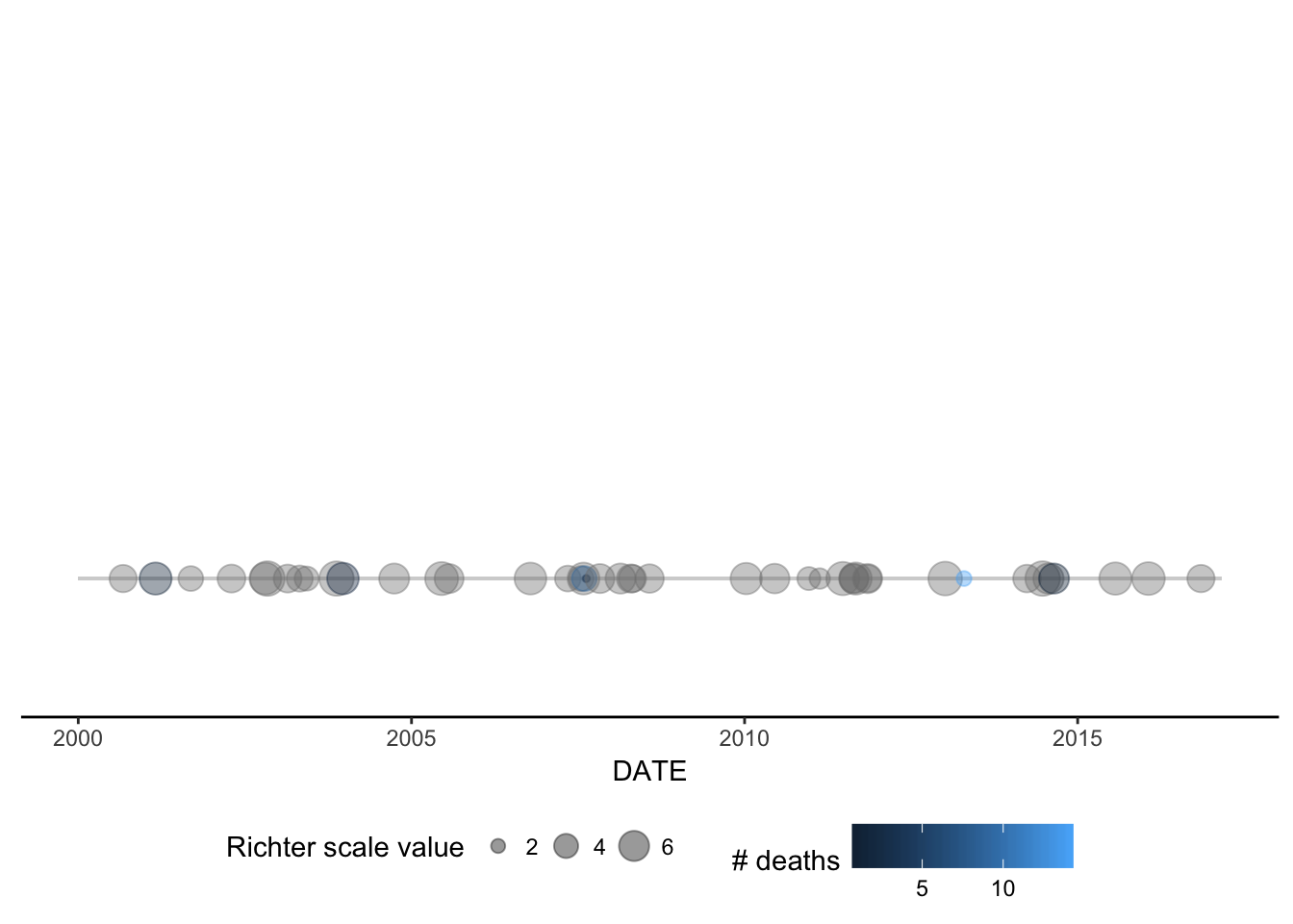
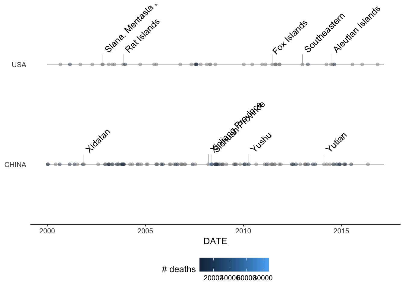
1. Build a geom for ggplot2 called geom_timeline() for plotting a time line of earthquakes ranging from xmin to xmaxdates with a point for each earthquake. Optional aesthetics include color, size, and alpha (for transparency). The xaesthetic is a date and an optional y aesthetic is a factor indicating some stratification in which case multiple time lines will be plotted for each level of the factor (e.g. country).

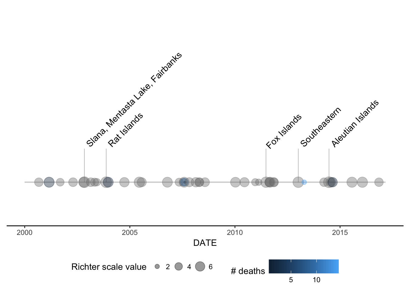
1. Build a geom called geom_timeline_label() for adding annotations to the earthquake data. This geom adds a vertical line to each data point with a text annotation (e.g. the location of the earthquake) attached to each line. There should be an option to subset to n_max number of earthquakes, where we take the n_max largest (by magnitude) earthquakes. Aesthetics are x, which is the date of the earthquake and label which takes the column name from which annotations will be obtained.

Week-3: Mapping Tools

In addition to building tools to visualize the earthquakes in time (as we did in the last module), it’s important that we can visualize them in space too. In this module we will build some tools for mapping the earthquake epicenters and providing some annotations with the mapped data.

Build a function called eq_map() that takes an argument data containing the filtered data frame with earthquakes to visualize. The function maps the epicenters (LATITUDE/LONGITUDE) and annotates each point with in pop up window containing annotation data stored in a column of the data frame. The user should be able to choose which column is used for the annotation in the pop-up with a function argument named annot_col. Each earthquake should be shown with a circle, and the radius of the circle should be proportional to the earthquake's magnitude (EQ_PRIMARY). Your code, assuming you have the earthquake data saved in your working directory as "earthquakes.tsv.gz", should be able to be used in the following way:

readr::read_delim("earthquakes.tsv.gz", delim = "\t") %>% 
  eq_clean_data() %>% 
  dplyr::filter(COUNTRY == "MEXICO" & lubridate::year(DATE) >= 2000) %>% 
  eq_map(annot_col = "DATE")

Which should produce the following result:

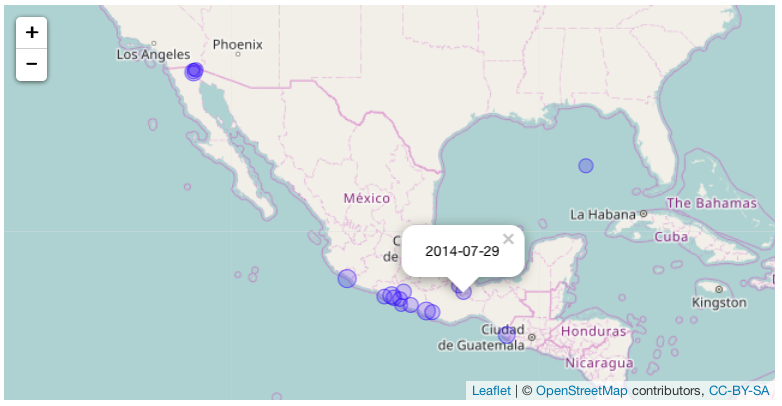
This is just an image, of course your result will be a fully interactive map.

Finally, it would be useful to have more interesting pop-ups for the interactive map created with the eq_map() function. Create a function called eq_create_label() that takes the dataset as an argument and creates an HTML label that can be used as the annotation text in the leaflet map. This function should put together a character string for each earthquake that will show the cleaned location (as cleaned by the eq_location_clean() function created in Module 1), the magnitude (EQ_PRIMARY), and the total number of deaths (TOTAL_DEATHS), with boldface labels for each ("Location", "Total deaths", and "Magnitude"). If an earthquake is missing values for any of these, both the label and the value should be skipped for that element of the tag. Your code should be able to be used in the following way:

readr::read_delim("earthquakes.tsv.gz", delim = "\t") %>% 
  eq_clean_data() %>% 
  dplyr::filter(COUNTRY == "MEXICO" & lubridate::year(DATE) >= 2000) %>% 
  dplyr::mutate(popup_text = eq_create_label(.)) %>% 
  eq_map(annot_col = "popup_text")

Which should produce the following result:

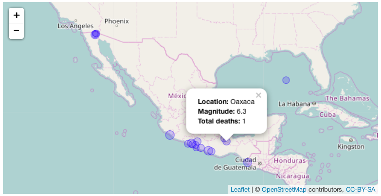
Again we're only able to show an image here but your result should be a fully interactive map.

Week-4: Documentation

Documentation and Packaging Tasks

Documentation is one of the most important and most commonly overlooked steps when writing software. You might be creating a revolutionary R package with code that is brilliantly implemented, but without clear and accessible documentation nobody will be able to use your package! In R packages there are two primary levels of documentation, the help files for individual functions and a vignette which contains a detailed explanation of how the package should be used, including examples featuring each function in the package. You should also consider writing a useful README.md file for your package so that when new users visit your package's GitHub repository they can quickly get the gist of how your package works.

In this module you should make sure to do the following:

• Make sure that every function in your package has appropriate help page documentation, including an example use for every function.

• Make sure your package has a DESCRIPTION, LICENSE, NAMESPACE, and README.md file.

• Write a vignette for your package that includes an explanation of the purpose for your package and how it could be used. The vignette should include examples for every function that is exported in the package's NAMESPACE file.

When you're finished with these tasks commit the changes to your package to GitHub so that you can show your package to your fellow students in the peer assessments.

Testing

Whenever developing software it's always important to write good tests for your functions. Tests ensure that your functions are behaving the way you expect them to behave. If you change your package in the future the tests that you've written will help you make sure that your changes didn't break any functionality.

In this module you should:

Use the testthat package to write at least one test for every function in your package. Use the devtools package to test your package on your computer.

Week-5: Your First Deployment

GitHub is the world's most popular code repository and it also functions as a great way to distribute your R package. Package users can easily install your package and look at's documentation if your package is on GitHub. With your package on GitHub you can take advantage of Travis for continuous integration. Each time you push new commits to GitHub, Travis will automatically rerun your tests!

In this module you should do the following:

Create a GitHub repository for your package and push your package code to GitHub. Configure Travis CI so that it tests your R package. You'll need to add a .travis.yml file to your package. Once you have Travis set up add your package repository's Travis badge to your package's README.md file. Make sure your package is building on Travis without any errors, warnings, or notes.

EnriquePH/NOAA.earthquake documentation built on May 6, 2019, 3:26 p.m.