In JGCRI/rfasst: rfasst

knitr::opts_chunk$set(
  collapse = TRUE,
  comment = "#>"
)

The functions that form this module estimate adverse agricultural impacts attributable to ozone exposure. These functions calculate relative yield losses (RYLs) and the subsequent production and revenue losses damages, combining O3 concentration data (see Module2 concentration), with agricultural production and price projections from GCAM.

RYLs are estimated for four main crops (maize, rice, soybeans, and wheat), using exposure-response functions (ERFs), and are calculated using two different indicators for O3 exposure: accumulated daytime hourly O3 concentration above a threshold of 40 ppbV (AOT40) and the seasonal mean daytime O3 concentration (M7 for the 7-hour mean and M12 for the 12-hour mean). These damges are then extended to the rest of the commodities based on their carbon fixation pathway, as explained below. For AOT40, RYLs are calculated with a linear function described in Mills et al (2007):

$$RYL_{t,r,j}=\alpha_j \cdot AOT40_{t,r,j} $$

For Mi, the exposure-response function is detailed in Wang and Mauzerall (2004) and follows a Weibull distribution (for $M_i$>$c$, 0 otherwise):

$$RYL_{t,r,j}=1-\frac{exp~[-(\frac{M_{t,r,j}}{a_j})^{b_j}]}{exp~[-(\frac{c_j}{a_j})^{b_j}]}$$

More information on the methodology used for the estimation of agricultural damages can be found in the TM5-FASST documentation paper (Van Dingenen et al (2018)) and in Van Dingenen et al (2009). The combined use of the models for estimating agricultural damages is explained in more detail in Sampedro et al (2020).

Production losses are calculated combining the RYLs with projected agricultural production levels of the analyzed GCAM scenario. In addition, multiplying the projected price by the production losses (quantities), we estimate revenue losses for period $t$, region $i$, and crop $j$ as:

$$Damage_{t,r,j}=Prod_{t,r,j} \cdot Price_{t,r,j} \cdot Pulse.RYL_{t,r,j}$$

As explained above, the module combines O3 concentration data with agricultural production and price projections. However, in order to complete all the calculations, the package includes some additional information:

2010 data on harvested area for downscalling the damages to country level in order to re-scale them to the corresponding regional disaggregation (d.ha;area_harvest.csv)
RYLs based on the different exposure-response functions are calculated for four main crops (maize, rice, soybeans, and wheat), so the damages need to be expanded to the rest of the commodities. The package includes a commodity mapping that expands the damages to all the crops based on their carbon fixation pathway (C3 or C4 categorization) (d.gcam.commod.o3; GCAM_commod_map_o3.csv)

We note that these two files could be easily modified by the user if any other mapping/downscalling technique is preferred. The files are stored in the /inst/extada/mapping folder.

Finally, all the functions that form this module provide the following list of outputs:

RYL_AOT40_[scenario]_[year].csv
RYL_Mi_[scenario]_[year].csv
PROD_LOSS_[scenario]_[year].csv-- These files include production losses using both the AOT40 and Mi indicators
REV_LOSS_[scenario]_[year].csv-- These files include production losses using both the AOT40 and Mi indicators

The code below shows some examples that show how to produce some of these outputs:

library(rfasst)
library(magrittr)

 db_path<-"path_to_your_gcam_database"
 query_path<-"path_to_your_gcam_queries_file"
 db_name<-"name of the database"
 prj_name<-"name for a Project to add extracted results to" # (any name should work, avoid spaces just in case) 
 scen_name<-"name of the GCAM scenario"
 queries<-"Name of the query file" # (the package includes a default query file that includes all the queries required in every function in the package, "queries_rfasst.xml")


  # To write the some outputs as csv files into the corresponding output folder:

    # Relative yield losses.
       Using AOT40 as O3 exposure indicator: m4_get_ryl_aot40(db_path,query_path,db_name,prj_name,scen_name,queries,saveOutput=T, map=F) 
       Using Mi as O3 exposure indicator: m4_get_ryl_mi(db_path,query_path,db_name,prj_name,scen_name,queries,saveOutput=T, map=F) 

    # Production losses (includes losses using both AOT40 and Mi).
       m4_get_prod_loss(db_path,query_path,db_name,prj_name,scen_name,queries,saveOutput=T, map=F) 

    # Revenue losses (includes losses using both AOT40 and Mi).
       m4_get_rev_loss(db_path,query_path,db_name,prj_name,scen_name,queries,saveOutput=T, map=F) 

#----------------------------------------------

  # To save this data by TM5-FASST region in year 2050 as dataframes:

    # Relative yield losses.
      # Using AOT40 as O3 exposure indicator:
         ryl.aot40.2050<-dplyr::bind_rows(m4_get_ryl_aot40(db_path,query_path,db_name,prj_name,scen_name,queries,saveOutput=F, map=F)) %>% dplyr::filter(year==2050)

      # Using Mi as O3 exposure indicator:
         ryl.mi.2050<-dplyr::bind_rows(m4_get_ryl_mi(db_path,query_path,db_name,prj_name,scen_name,queries,saveOutput=F, map=F)) %>% dplyr::filter(year==2050)

    # Production losses (includes losses using both AOT40 and Mi).
       prod.loss.2050<-dplyr::bind_rows(m4_get_prod_loss(db_path,query_path,db_name,prj_name,scen_name,queries,saveOutput=T, map=F)) %>% dplyr::filter(year==2050)

    # Revenue losses (includes losses using both AOT40 and Mi).
       rev.loss.2050<-dplyr::bind_rows(m4_get_rev_loss(db_path,query_path,db_name,prj_name,scen_name,queries,saveOutput=T, map=F)) %>% dplyr::filter(year==2050)

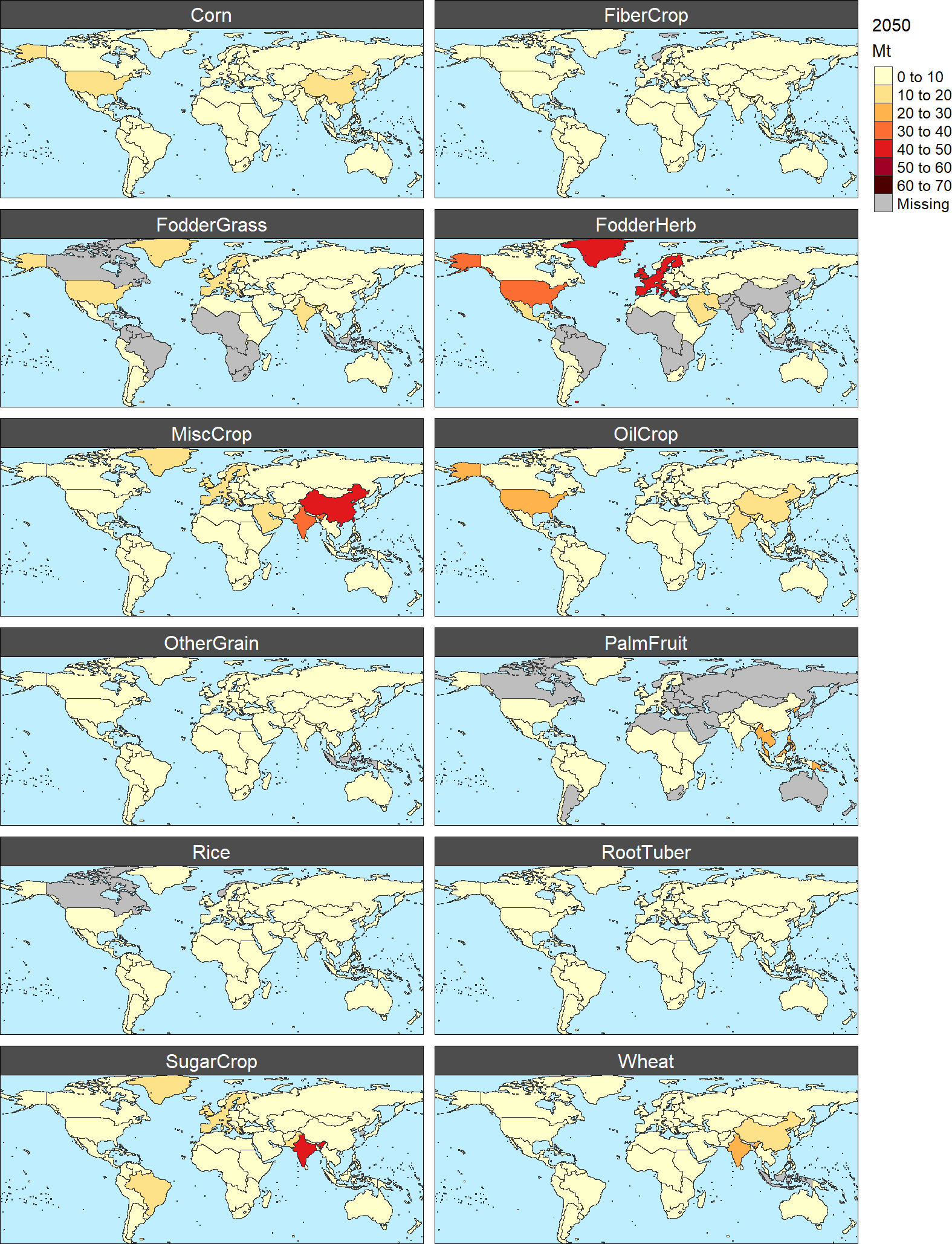
As in Modules 2 and 3, for all these functions, the package allows to produce different figures and/or animations, generated using the rmap package documented in the following page. To generate these maps, the user needs to include the map=T parameter, and they will be generated and stored in the corresponding output sub-directory. As an example for this module, the following map shows the production losses attributable to O3 exposure in 2050.

*Agricultural production losses attributable to O3 exposure by commodity in 2050 (Mt)*