inst/examples/manuscript.md

In cboettig/wrightscape: wrightscape

• Author: Carl Boettiger [e-mail]
• License: BSD

require(wrightscape)
require(ggplot2)
require(reshape)
data(labrids)

traits <- c("bodymass", "close", "open", "kt", "gape.y", "prot.y", 
    "AM.y")
regimes <- two_shifts

nboot <- 100
cpu <- 16

require(snowfall)
sfInit(parallel = TRUE, cpu = cpu)

R Version:  R version 2.15.0 (2012-03-30) 

sfLibrary(wrightscape)

Library wrightscape loaded.

sfExportAll()

Fit all models, then actually perform the model choice analysis for the chosen model pairs

fits <- lapply(traits, function(trait) {
    multi <- function(modelspec) {
        multiTypeOU(data = dat[[trait]], tree = tree, regimes = regimes, model_spec = modelspec, 
            control = list(maxit = 8000))
    }
    bm2 <- multi(list(alpha = "fixed", sigma = "indep", theta = "global"))
    a2 <- multi(list(alpha = "indep", sigma = "global", theta = "global"))

    mc <- montecarlotest(bm2, a2, cpu = cpu, nboot = nboot)
})

require(reshape2)
require(ggplot2)

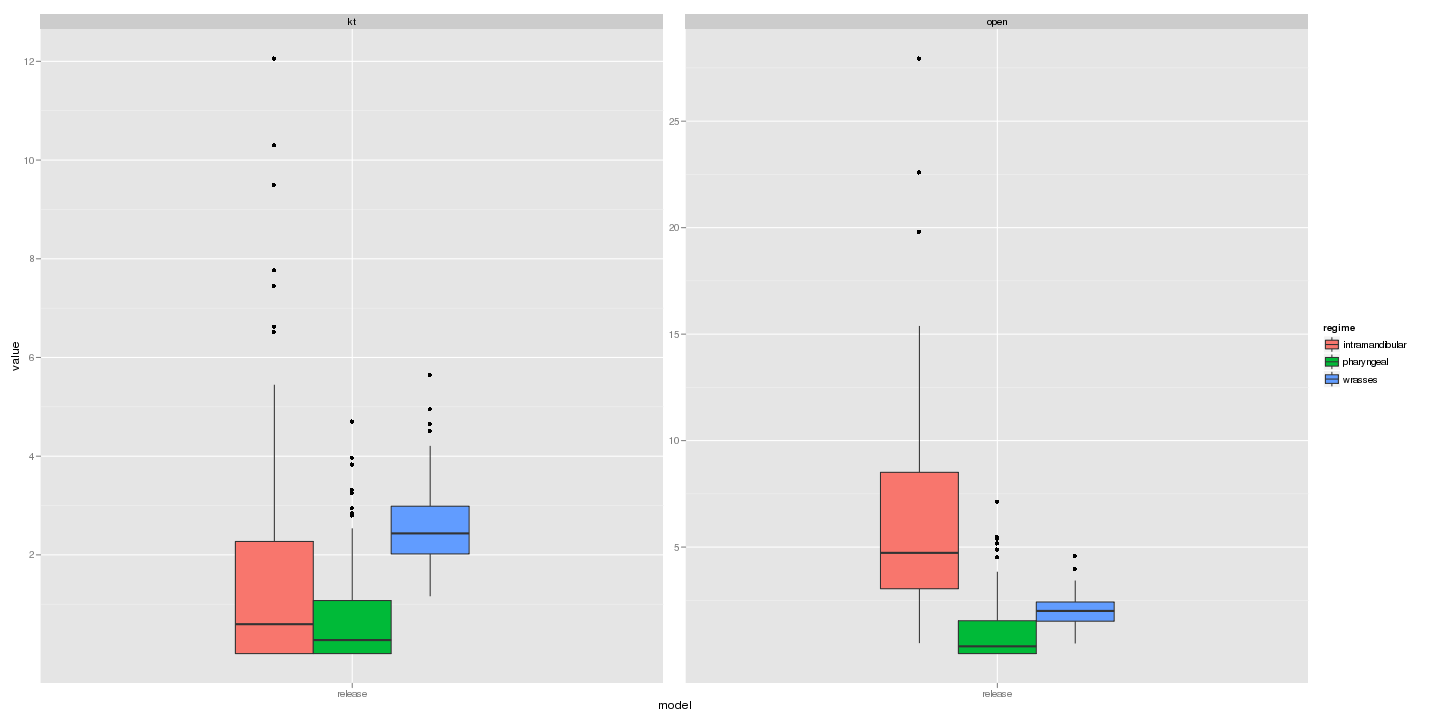
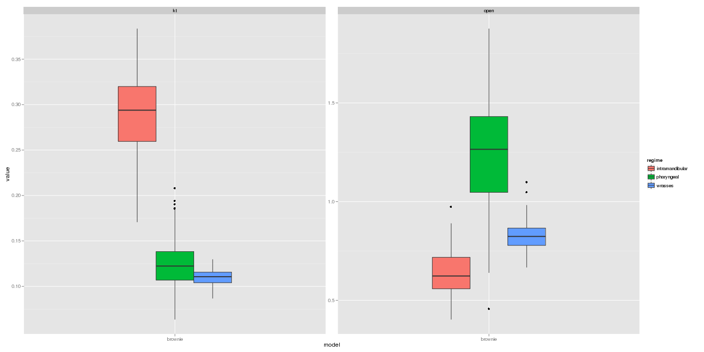
Parameter distributions

regroup <- function(df) {
    df <- as.data.frame(t(df))
    alpha <- df[c("alpha1", "alpha2", "alpha3")]
    sigma <- df[c("sigma1", "sigma2", "sigma3")]
    theta <- df[c("theta1", "theta2", "theta3")]
    names(alpha) <- levels(fits[[1]]$null$regimes)
    names(sigma) <- levels(fits[[1]]$null$regimes)
    names(theta) <- levels(fits[[1]]$null$regimes)
    # , Xo = df$Xo, converge=df$converge
    list(alpha = alpha, theta = theta, sigma = sigma)
}
dat <- melt(list(open = list(brownie = regroup(fits[[1]]$null_par_dist), 
    release = regroup(fits[[1]]$test_par_dist)), kt = list(brownie = regroup(fits[[2]]$null_par_dist), 
    release = regroup(fits[[2]]$test_par_dist))))
names(dat) <- c("regime", "value", "parameter", "model", "trait")

ggplot(subset(dat, model == "release" & parameter == "alpha")) + 
    geom_boxplot(aes(model, value, fill = regime)) + facet_wrap(~trait, scale = "free_y")

ggplot(subset(dat, model == "brownie" & parameter == "sigma" & value < 
    2)) + geom_boxplot(aes(model, value, fill = regime)) + facet_wrap(~trait, 
    scale = "free_y")

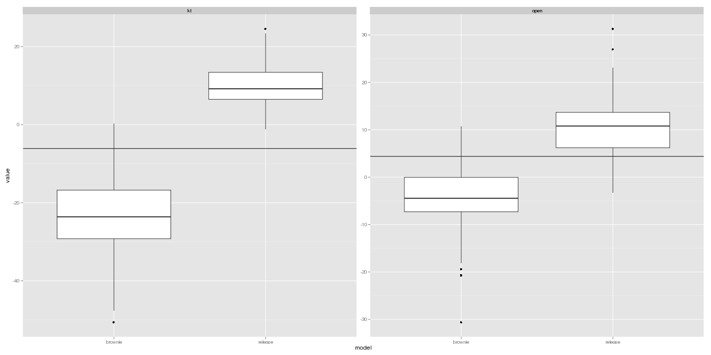
Likelihood ratio distributions:

lr_dat <- melt(list(open = list(release = fits[[1]]$test_dist, brownie = fits[[1]]$null_dist), 
    kt = list(release = fits[[2]]$test_dist, brownie = fits[[2]]$null_dist)))
open_LR <- 2 * (fits[[1]]$test$loglik - fits[[1]]$null$loglik)
kt_LR <- 2 * (fits[[2]]$test$loglik - fits[[2]]$null$loglik)
LR <- data.frame(value = c(open_LR, kt_LR), model = "ratio", trait = c("open", 
    "kt"))
names(lr_dat) <- c("value", "model", "trait")

ggplot(subset(lr_dat, value > -10000 & value < 10000)) + geom_boxplot(aes(model, 
    value)) + facet_wrap(~trait, scale = "free_y") + geom_hline(data = LR, aes(yintercept = value))

save(list = c("lr_dat", "dat", "fits"), file = "manuscript.rda")

cboettig/wrightscape documentation built on May 13, 2019, 2:12 p.m.