In dswdejonge/TripleD: Construct a TripleD database.
library(TripleD)
Short summary
- The NIOZ Royal Netherlands Institute for Sea Research owns a special dredge called the Triple-D (Deep Digging Dredge) to sample megafauna from sedimentary habitats.
- Data collected over the years, so far only from the North Sea, are stored in CSV files in the NIOZ Data Archiving System (DAS).
- The goal of the TripleD package is to read the CSV files, and employ pre-written workflows to obtain two database-style tables with 1) presence-absence, density, and biomass data, and 2) individual size and weight data of benthic megafauna.
- The transparancy and elaborate documentation allows users of the package to exactly retrace the source of data, how calculations were performed, and which assumptions underly the data in the final database.
- This workflow also allows the user to rewrite (part of) the workflow to process the original data if they have specific wishes/assumptions they would like to use.
- The output of the TripleD package can directly be used in a developed Shiny app to visually interact with the data.
Citation
Please use the citation specified for each individual dataset.
1. Introduction
The Triple-D (Deep Digging Dredge) is a dredge designed by NIOZ Royal Netherlands Institute for Sea Research that can easily sample relatively large areas of seabed to quantitatively study the distribution of megafauna that generally occurs in low abundances. So far, the Triple-D is only used in the North Sea, mostly on the Dutch Continental Shelf.
The Triple-D was introduced in the last century and has been happily sampling every since. The data collected over the years forms a valuable time series and it was decided to more systematically archive the data to allow easier exploration of this wealth of data and easier incorporation of new data in the future. This Triple-D R-package is the result of this decision, and this vignette explains why.
The basic idea is three-fold:
- All original sampling data is collected in CSV files (one file per research cruise) formatted in a specific way as specified by the Triple-D package. This data is original data, meaning with as few underlying assumptions as possible. This original data - that should not be mutated - is archived in the NIOZ Data Archiving System (DAS). The data is owned by NIOZ and can be requested by potential users.
- The TripleD R-package can read the CSV files with original data, and processes this data using pre-written workflows to produce a single database-like table with presence-absence, density, and biomass data that can be used in ecological analyses. So, by running the package with requested CSV files you can construct a local database on your own machine. The R-package is available to everyone with completely transparent workflows and elaborate documentation. Therefore, the user is able to completely retrace all data mutations and can even re-write (part of) the workflow if (s)he wishes to produce a personal database that uses other calculations and assumptions from the default workflow.
- A Shiny app is developed to visually interact with the database as produced by the default workflow in the TripleD package. It allows the user to intuitively filter and browse the data in order to better grasp what data is available, and how the data can be employed for the research question at hand.
This vignette contains background information on the Triple-D itself, explains how to use the Triple-D package, and provided guidelines how you can add new data to the Triple-D data archive.
Acknowledgements
Magda Bergman
Rob Witbaard
Marc Lavaleye
Dick van Oevelen
2. The Triple-D: Deep Digging Dredge
2.A. Description
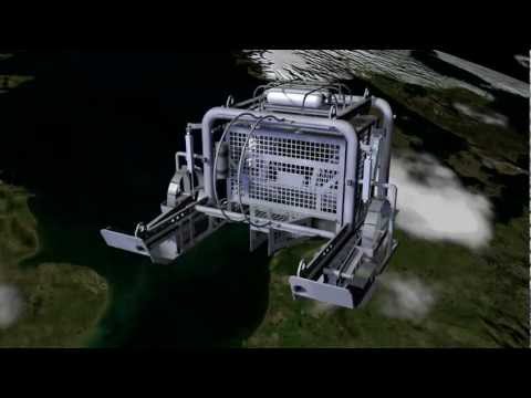
A prototype of the Triple-D was introduced by Bergman & Santbrink [@Bergman1994]. It was developed in order to better quantitatively study the distribution of generally sparsly abundant megafauna. The prototype Triple-D was 2.0 m long, 1.5 m wide and 1.5 m high and weighted about 600 kg. The current Triple-D is 2.4 m long, 2.6 m wide, 1.2 m high and weights about 1200 kg. The dredge contains a blade of 20 cm width that is pushed into the sediment to a depth of 20 cm and consequently towed over the seabed at a speed of 3 knots. The tow track length is measured by an odometer (a wheel tracking the distance) set to 100 m that also controls the pneumatic opening-closing mechanism. The sediment that is exised from the seabed passes through a tailing 6 m with a mesh size of 7 mm. The remaining fauna in the net representing a total area of 20 m2 are brought aboard for identification and measurements.
More information: http://ipt.nioz.nl/resource?r=triple-d_dredge
Video:
2.B. Sampling procedure
The dredge is lowered to the seabed and towed over the sediment until it's stable (the pre-track distance). The blade is pushed into the sediment to start the actual sampling track in a certain direction (bearing). The length of this sampling track is preset, and often 100 m (especially in recent years). All sediment exised by the blade pass through a net that retains the organisms. After the intended track distance the blad is taken out of the sediment, and the catch is brought up to the ship. Based on several sources of information it is decided whether or not the sampling track was successful and can be used quantitatively.
On board, any remaining sediment is washed from the organisms. The organisms are identified and grouped. Preferably all specimens are counted, measured, and weighed. However, due to the sometimes large number of specimens only a representative fraction of the species is measured and weighed. For example, 100 specimens of Asterias rubens (common sea star) are caught. Due to time constraints, 20 representative specimens are selected, measured and weighed (the other 80 are discarded). These measurements (size and weight) are noted together with a fraction of 0.2 (i.e. 20 of 100 specimens processed). This fraction is later used to upscale the measured values to an estimation for the complete catch.
If you want to use the TripleD to collect organisms, follow these guidelines to easily convert your documented work into data for the TripleD database:
1) For each research cruise eventually a stations CSV data file, a species CSV data file, and a readme text file should be created. Take a look at the required attributes and detailed definitions first (see 3.B.). You can even create and print a template sheet to fill in your data while working onboard.
2) Write down the specs of the TripleD: What blade depth and width are you using? What is your net mesh size? And other important information. Document this as explained in the attributes file.
3) Decide beforehand if you are going to process the full catch, or if you are going to ignore certain groups? Perhaps you only want to study a certain group (e.g. bivalves) and you will ignore the rest. Document this as explained in the attributes file.
4) While sampling, keep good track of the date, time (UTC+0), and position (WGS84) of the ship and the dredge track. Preferably also document other information like tow speed, bearing, and water depth.
5) When the TripleD is back on board, assess the confidence of the sampled track. If something appears to have gone wrong, document this. If the catch cannot be used quantitatively, but the information is usefull for presence-absence or relative abundances withint the sample, document this as explained in the attributes files.
6) Identify and sort the catch. The process will be smoother if the full catch is properly sorted before starting the measurements. You can document who identified the species and if that identification is confident (i.e. no doubt).
7) Preferably, each individual is measured and weighed. However, sometimes it is easier to pool some organisms together. For example, if multiple organisms have the same size, you can decide to pool and weigh them together. Report how many specimens are included in each entry (count). Egg masses, and algae batches, and other loose material that you want to document, should be reported with a count of -1. Each entry must have a unique ID. You can start assigning these onboard already. This is especially usefull when you want to store the organisms for later analysis in the lab (e.g. AFDW measurements). Make sure to consistently use this ID! Document if you will preserve certain organisms and where a user of the database may find these specimens in the future.
7) For each taxon, measure the size of all organisms. Carefully document the size dimension measured (diagram below), the unit (mm, cm, 1/2cm [note on using 1/2cm units below]), and the value. You can also only process a fraction of the catch, document this accordingly. Below is a diagram that explains for each general morphological group what size dimensions may be measured and what unit is the most appropriate. Hanging this diagram onboard as a large A1 poster, and providing it as laminated hand-out may help your colleagues/studnets/volunteers in the process. Sticking to the defined size dimensions and documenting their names strictly as written on the diagram will ease digitizing your measurements!
knitr::include_graphics("https://raw.githubusercontent.com/dswdejonge/TripleD/master/inst/extdata/_morphologies.png")
8) For each taxon: weigh the wet weight. You can also only process a fraction of the catch, document this accordingly. Document the threshold of the scale you are using. If the weight of a specimen is below the threshold, record 0. If the weight is not measured at all, record NA. If an organism is broken/missing body parts, write down that the wet weight is an underestimation because it only concerns a partial wet weight. If an organism naturally occurs with a hard external structure, like a shell (also hermit crabs!) or a tube (tube worms), write down if this shell was removed before weighing! If your weight does NOT concern a single entry but is a bulk weight (e.g. all specimens of a certain taxon are weighed together but measured for size seperately), document this accordingly! Eggs should generally not be included in the weight and be weighed seperately, unless it can't be avoided.
9) If you decide to take specimens back to the lab (read point 6!) for ash-free dry weight (AFDW) measurements, also document the scale threshold, if the organisms were broken, and if the weight is a bulk weight or not. AFDW is the dry weight (drying of wet tissue in the oven) minus the weight of the ash left after combustion of the tissue, i.e. AFDW and dry weight are not equivalent. Ash-free dry weight only concerns biologically active tissue, so external hard structures like shells are always removed. Make sure you match the AFDW measurement to the right entry (use the unique entry IDs). AFDW is the measurement type used to report final biomasses in the database.
Following these guidelines should make it easy to digitize your data as required by the TripleD package (see 3.B.).
knitr::include_graphics("https://raw.githubusercontent.com/dswdejonge/TripleD/master/inst/extdata/half_cm_units.png")
Note on using the 1/2cm unit:
The unit 1/2cm is used a bit differently than the units mm and cm, because it works with ‘classes’. Imagine you have a ruler with tick-marks every 5 mm. So, the first tick mark at 0 mm, the second tick mark at 5 mm, the third tick mark at 10 mm, etc. If the organism is at least 5 mm (so between 5 and 10 mm) it falls in the class 1 ½cm. This means that an organism that is 4 mm falls in the class 0 ½ cm,and an organism of 14 mm will fall in the class 2 ½cm. Understanding this system is especially important if you want to convert ½units to mm or cm.
2.C. Limitations
- The blade width and blade depth dimension are the intended sampling width and depth. However due to sediment types, objects in the sediment, and unevenness of the sediment, the actual track width and depth may differ somewhat. No study is yet done to quantify these effects.
- Polychaetes are caught by the Triple-D, but the Triple-D is not suitable for a quantitative analysis of polychaete abundance.
- Amphiura are often broken when processed, therefore the measured wet weights are probably almost always underestimations.
- Species identification might have changed throughout time. For example, species A might have been identified as such, until at a certain moment in time it was recognized species A was in fact two different species, species A and B. It is important to be aware of such historic artefacts when working with and interpreting the data.
3. The TripleD R-package
3.A. Quick start
The Triple-D R-package and all related files can be found in its GitHub repository: github.com/dswdejonge/TripleD. Go to the readme file in the repository for guidance on 1) installing the package, 2) seting up your working directory, and 3) running the workflow.
Cheatsheet
The general structure of the package, and how files relate to each other, are explained in this cheatsheet:
knitr::include_graphics("https://raw.githubusercontent.com/dswdejonge/TripleD/master/inst/extdata/cheatsheet.png")
Error handling
If you encounter errors, try the advice below.
construct_database() expects double but finds integer
You may get an error during the construct_database() function where a double is expected (e.g. 1.00) but an integer (e.g. 1) is found. Open the CSV file in Excel, select all columns that should be doubles, and set the datatype to 'Number' (all vallues should get the format 1.00 instead of 1). Save and try again.
Input files invisible characters
CSV files are basically text files where information that should occur in separate columns are separated by a comma (csv = comma separated values). Sometimes, text files can contain invisible characters that will create issues when trying to use it in R. If you suspect such issues might occur (you will probably get errors in the construct_database() function) try the following:
A. Encoding of File
The file encoding tells the computer how it should represent the text so that it is readable. Some issues with reading and using a text file might occur due to differences in file encodings. The file encoding I have used for the CSV files is UTF-8. You can use a free text editor like Notepad++ or SublimeText to reopen and store a file in a certain encoding.
B. Byte Order Mark (BOM)
A Byte Order Mark (BOM) is an invisible character that is sometimes added right at the start of a file. This is done for example by Microsoft Excel. However, R does not like this BOM when reading in a CSV and adds the characters to the first column name (something like “StationID”). To avoid this, you can use a text editor to specifically change the encoding of the file to “UTF-8 without BOM”.
C. Spaces
Spaces are exactly what the word says: invisible space between words. However, there are multiple characters that create space between words and differ from regular spaces. It might occur, for example, that you accidentally used a tab instead of a space. Also, there are special spaces called ‘non-breaking spaces’ that are the same as a normal space except that they prevent an automatic line break. If a regular space is “_”, a tab is “” and a non-breaking space is “^” you get the following problem:
Genus_species is not the same as Genusspecies or Genus^species. In other words, on screen the statements appear exactly the same for the user, but the computer sees them as different characters. If you think you might have alternative spaces in your CSV, use a text editor to search and replace tabs and non-breaking spaces with regular spaces.
Connection time-out
The functions collect_from_NOAA and collect_from_WORMS contain clients that try to connect to the API of external databases. It may occur that, for whatever reason, the connection is lost. You may get an error like this:
Error in curl::curl_fetch_memory(x\$url\$url, handle = x\$url\$handle) :
Timeout was reached: [www.marinespecies.org] Connection timed out after 10003 milliseconds.
If this is the case, simply try running the function again, as it might have simply occurred due to a hiccup in your or the server’s internet connection.
3.B. Input files
The TripleD package can only read in CSV data files - one with sampling station data and one with species data per research cruise - that meet the specified requirements. The attribute files included in the package describe these requirements. This may require cleaning of your raw data files. A description of this cleaning process must be logged in the corresponding readme file.
Preparation of the CSV files is best done manually: it can be the step where you carefully review the data you noted during the cruise (e.g. on paper) while you convert it to a carefully documented digital format.
General requirements:
- Per research cruise you need three files: 1) Station data ('Year_CruiseID_stations.csv'), 2) Species data ('Year_CruiseID_species.csv'), and 3) a readme file explaining how the former two files were constructued ('Year_CruiseID_README.txt').
- As much as possible, only include original data, i.e. measured and derived during the research cruise, and not calculated or sourced from an external dataset.
- Fields may never be empty.
- Always be aware of the difference between 'NA' (not measured) and '0' (measured and value is 0).
- A sampling station corresponds to a single unique sampling event (i.e. dredge track), and NOT to a geographical location.
- CruiseID, StationID, and EntryID are always required and must contain unique values. StationID is especially important because it is used to match station data to species data.
- Do not include columns where all values are NA (otherwise R will treat them as characters in stead of missing values).
- Following from the former statement, it is not necessary to include all columns in the attributes files. The attributes files note which columns are 'Required' (i.e. they must always be included) and which are 'Optional' (i.e. if you haven't measured this data, simply leave this column out).
- Coordinates must be in WGS84.
- Time must be in UTC+0.
- Please report in English as much as possible, so that international researchers can also use the data.
Stations CSV attributes can be viewed here, and species CSV attributes can be viewed here. Alternatively, you can view the requirements in R:
library(TripleD)
print(att_stations)
print(att_species)
To help guide you with constructing the CSV files according to the requirements, I have added some examples below. Don't forget to write a readme file with a log of how you constructed your CSV files!
Example: Stations name
Entry for a cruise 64PE330 in 2017 for a project called FakeSamples. The third sampling track was within a windmill park at a fixed monitoring station called WM10.
|CruiseID | StationID | Date | Cruise_name | Station_name | Region | Comment |
| ------- | --------- | ---------- | ----------- | ------------ | ------ | ------- |
|64PE330 | 64PE330#3 | 01/01/2017 | FakeSamples2017 | WM10 | WM | Monitoring station |
Note that the CruiseID (required) and Cruise_name (optional) should not be confused, just like StationID (required and used to match to the species file) and Station_name (optional). The date should be in the correct format (01-01-2017 would be wrong), and the region should be a predefined abbreviation in the attributes file.
Example: Coordinates and time
During cruise 64PE330 you sampled a station and recorded the start and stop coordinates of the track in coordinate system ED50 i.e. EPSG4230 (e.g. 5.2185, 54.329 to 5.2180, 54.322), and the local start and stop time (16.30 - 17.00 UTC+2).
devtools::install_github("dswdejonge/rgis")
library(rgis)
rgis::transform_latlon_to_different_CRS(data.frame(x= c(5.2185, 5.2180),
                                                   y = c(54.329, 54.322)),
                                        epsg_code_from = 4230, epsg_code_to = 4326)
| StationID | Lat_start_DD | Lon_start_DD | Lat_stop_DD | Lon_stop_DD | Time_start | Time_stop |
| --------- | ------------ | ------------ | ----------- | ----------- | ---------- | --------- |
| 64PE330#4 | 54.32828 | 5.217122 | 54.32128 | 5.216622 | 14:30:00 | 15:00:00 |
Note that the coordinates are always expected in coordinate reference system WGS84 (aka EPSG:4326), meaning that in this case the coordinates reported in ED50 (aka EPSG:4230) must first be transformed. In this case I used a function written in R hosted on GitHub, but there is also a web functionality that can be used (https://epsg.io/transform). Also note that the reported time must always have the format HH:MM:SS (so 14.30 would not be accepted) and must be reported in UTC+0, meaning in this case the time had to be converted from local time UTC+2 to UTC+0. In your readme file you should state how you converted your original data to fit the requirements of the TripleD CSV files! Finally, you should either provide start and stop coordinates of the track OR the track midpoint coordinates, i.e. at least of of them is required. You are free to add both pieces of information but it is not necessary (the TripleD package can automatically calculate track length and midpoint based on the provided start and stop coordinates).
Example: Sample metadata
After retrieving the net it was found to be overfull, mostly due to Calianassa mud shrimp and Abra alba bivalves. It is decided to do another track right beside the original track, but at only half of the original track length and disregarding Calianassa and Abra alba entirely. This time the retrieved net is not overfull.
| StationID | Track_length_m_preset | is_Quantitative | Station_objective | Excluded |
| --------- | --------------------- | --------------- | ----------------- | -------- |
| 64PE330#4 | 100 | 0 | Complete | NA |
| 64PE330#5 | 50 | 1 | Incomplete | Calianassa;Abra alba|
As the first net was overfull, the catch cannot be used quantitatively (i.e. to calculate density or biomass per m2 or m3), however, the information is kept for e.g. studying relative abundance within this one catch. The second track was much shorter, and therefore the catch can be used quantitatively. However, during later ecological analysis it must be taken into account Calianassa and Abra alba were excluded in processing the catch (i.e. the lack of those species in this specific sample does not mean they weren't present). Note that the species in the column 'Excluded' are seperated with a ';'.
Example: Water depth
You lost the notes with water depth for some stations measured during the research cruise. However, you do have a bathymetric map with water depths on which you can find depths based on the coordinates.
| StationID | Water_depth_m_cruise | Comment |
| --------- | ---------------------| ------- |
| 64PE330#4 | 32 | NA |
| 64PE330#5 | NA | Water depth notes lost |
| 64PE330#6 | NA | Water depth notes lost |
Only include original data in your dataset as much as possible. Therefore, you should set the missing water depth values to NA and not include calculated water depths based on the bathymetric map. Instead, you can use your bathymetry data in the package to automatically derive water depth at the track midpoints during the package workflow. Beware that if no water depth is recorded at all, i.e. the full column will be set to NA, do not include a water depth column as R will read this column to be full of characters 'NA' instead of numeric.
Example: Species presence
You sampled with the TripleD, and now want to record which species you found with the minimum of required fields.
| StationID | EntryID | Species_reported | Fraction | is_Fraction_assumed |
| --------- | ----------- | ----------------- | -------- | ------------------- |
| 64PE330#4 | 64PE330#4_1 | Asterias rubens | 1 | 0 |
| 64PE330#4 | 64PE330#4_2 | Abra alba | 1 | 0 |
| 64PE330#4 | 64PE330#4_3 | Crangon crangon | 1 | 0 |
| 64PE330#4 | 64PE330#4_4 | Lanice conchilega | 1 | 0 |
These are the minimum number of required fields to report species sampled with the TripleD. The StationID is used to match the biological data to the station data (not reported in the other examples for brevity). The EntryID denotes every unique entry. The Species_reported is the name of the species found at that sampling station. The Fraction and is_Fraction_assumed are always required, even if you don't report counts, sizes, or weights. In this case you wrote down presence based on the whole catch so the Fraction is 1 and it is not an assumed fraction (=0). Using the data becomes a lot more fun if counts, sizes, and weights are also reported (see other examples).
Example: Taxon identification
You found a couple of bivalve Ensis specimens that you cannot fully identify, they are either Ensis ensis or Ensis siliqua.
Option 1
| EntryID | Species_reported | is_ID_confident | ID_by | is_Preserved | Comment |
| ----------- | ---------------- | --------------- | ----- | ------------ | ------- |
| 64PE330#4_1 | Ensis sp. | 1 | D. de Jonge | 1 | A comment |
Option 2
| EntryID | Species_reported | is_ID_confident | ID_by | is_Preserved | Comment |
| ----------- | ---------------- | --------------- | ----- | ------------ | ------- |
| 64PE330#4_1 | Ensis siliqua | 0 | D. de Jonge | 1 | A comment |
If you are not sure about the taxonomic identification, the best option is to report the taxonomic level you are sure about. In other words, species names are preferred in the column 'Species_reported' but other taxonomic levels are also allowed as long as the scientific name is used. In the example under consideration you are sure the bivalve belongs to the genus Ensis so you report Ensis sp. (could also simply be Ensis, but avoid Ensis spec. or Ensis species as the taxa matching algorithm does not like this notation).
If you are almost sure about an identification, but not quite, you may choose to report the taxon you think it correct but identify your doubt about the identification in the column 'is_ID_confident'. It is best practice to store specimens with unsure ID, so that later identification in the lab can take place e.g. through barcoding. You can identify specimens that are stored in the column 'is_Preserved' and use the comment section to write where to find the stored sample (e.g.Stored in -20 NIOZ freezer under sample number '64PE330#4_1a').
Example: Specimen counts
In your full catch you find 10 sea stars Asterias rubens, 5 specimens of shrimp Crangon crangon, an egg mass of Abra alba, and a large clump of tube worms Lanice conchilega.
| EntryID | Species_reported | Fraction | is_Fraction_assumed | Count | Comment |
| ----------- | ----------------- | -------- | ------------------- | ----- | ------- |
| 64PE330#4_1 | Asterias rubens | 1 | 0 | 10 | NA |
| 64PE330#4_2 | Abra alba | 1 | 0 | -1 | Egg mass |
| 64PE330#4_3 | Crangon crangon | 1 | 0 | 5 | Snouts |
| 64PE330#4_4 | Lanice conchilega | 1 | 0 | NA | Large clump |
Some species are easily counted and reported. For some species, like Lanice conchilega, counting is sometimes omitted. In the latter case, you do want to report the presence but without counts, so the column 'Count' is set to NA, i.e. not to zero (it is recommended to include biomass in these cases, examples below). If you observe any items of interest which are not specimens (like egg masses or algae batches), set the count to -1 (again not to zero). Use the 'Comment' column to provide additional insight into your specimens and notations.
Example: Reporting fractions
In a sample, 20 sea stars Asterias rubens were found, but only 4 representative specimens were measured and weighed.
| EntryID | Species_reported | Fraction | is_Fraction_assumed | Count |
| ----------- | ---------------- | -------- | ------------------- | ----- |
| 64PE330#4_1 | Asterias rubens | 0.2 | 0 | 1 |
| 64PE330#4_2 | Asterias rubens | 0.2 | 0 | 1 |
| 64PE330#4_3 | Asterias rubens | 0.2 | 0 | 1 |
| 64PE330#4_4 | Asterias rubens | 0.2 | 0 | 1 |
Note that the reported 'Fraction' is the overall fraction of the catch of the reported species that was processed i.e. 4/20. It is NOT the fraction that each specimen makes up (1/20). You specifically noted the fraction, so the fraction is not assumed (=0). If you are not sure about the fraction, and you have to estimate this afterwards, it would have been 1. Also note that the counts are not yet corrected for the fraction.
The columns with potential size and weights are omitted in this example.
Example: Size measurements
You process 4 specimens of the seastar Asterias rubens (like the previous example) of different sizes, of which one is missing some arms. You also process 13 specimens of Abra alba, of which 5 specimens fall within the same size class, another 6 fall within the same size class, and you find two siphons without complete shells. You found a large clump of tube worms Lanice conchilega which you did not count, but you did estimate the volume of the colony. You also found a large specimen of the squid Alloteuthis sp. of which you measured both the mantle length and the length including tentacles.
| EntryID | Species_reported | Count | Size_dimension | Size_unit | Size_value | Comment |
| ----------- | ---------------- | ----- | -------------- | --------- | ---------- | ------- |
| 64PE330#4_1 | Asterias rubens | 1 | Max_length | cm | 9 | NA |
| 64PE330#4_2 | Asterias rubens | 1 | Max_length | cm | 9 | NA |
| 64PE330#4_3 | Asterias rubens | 1 | Max_length | cm | 8 | NA |
| 64PE330#4_4 | Asterias rubens | 1 | Disc_diameter | cm | 4 | Missing arms |
| 64PE330#4_5 | Abra alba | 5 | Shell_length | 1/2cm | 0 | NA |
| 64PE330#4_6 | Abra alba | 6 | Shell_length | 1/2cm | 1 | NA |
| 64PE330#4_7 | Abra alba | 2 | Siphon_width | mm | 3 | Broken |
| 64PE330#4_8 | Lanice conchilega | NA | Volume | cm3 | 13 | Large clump |
| 64PE330#4_9 | Alloteuthis sp. | 1 | Mantle_length | cm | 12 | Body length incl. tentacles = 19 cm |
Recording size measurements is a bit more complex than recording counts. You always need three grouped attributes: Size_dimension (describing what morphology was measured), Size_unit (describing what unit the value is in), and Size_value (the actual measured size value). The Size_dimension is important, because it determines which regression formula can be used to estimate biomass from the reported size.
You can report one size value per specimen (in the case of Asterias rubens in this example), or you can report a size value for a group of specimens (in the case of Abra alba in this example).
You can report different size dimensions and size units for one species if necessary. In this case example some Asterias rubens specimens are measured arm tip to arm tip (Max_length) whereas for one specimen the disc diameter is measured (Disc_diameter) because arms were missing in this specific broken organism. Also, for some specimens of Abra alba the Shell_length is measured in 1/2cm, and the Siphon_width is measured in mm for two broken specimens.
Beware of the use of 1/2cm as unit: it describes size classes (read the note under 2.B.), and it allows a size class of 0 1/2cm which does not mean 'no size' but 'between 0 and 5 mm'. If you did not measure a specimen, simply put 'NA' in all three size related columns.
This format does not allow the specification of multiple sizes for one specimen; each entry must really only represent the number of counted organism reported. In this example, two sizes are known for the squid Alloteuthis sp.. However, only one size can be reported (in this case it was chosen to report Mantle_length as official size, and note the other measurement in the comments). Reporting both sizes would require an additional entry, with the interpretation that two specimens were caught, which is not correct of course.
For some species, like sponges, tunicates, and colony-forming organisms, it is difficult to identify and measure a specific size dimension. In this cases it is possible to report (an estimated) area (in mm2 or cm2) or volume (in mm3 or cm3).
Example: Wet weight measurements
The specimens under 'Example: Size measurements' were also weighed. Additionally you weigh a hermit crab Pagurus bernhardus that was retrieved without a shell, six specimens of Arctica islandica for a study of size-weight relationships (shell lengths are already recorded to be 1, 1, 2, 2, 3 and 3 cm), and 10 large Ensis ensis specimens. A while later you find three additional Ensis ensis specimens you initially missed because they are smaller. You manage to measure their sizes, but do not have time to weigh them. You use a scale that can only record weights of 0.5 g or larger.
You find that all four specimens of Asterias rubens (of which one was missing some arms) together have a wet weight of 15 g. You find that the 11 complete specimens of Abra alba together weigh 7 grams, and that the 2 siphons with some shell remains together weigh less than the scale threshold (i.e. an exact weight cannot be determined). The Lanice conchilega colony is 102 grams. The Alloteuthis sp. individual is accidentally discarded before it could be weighed. The individual of Pagurus bernhardus that was retrieved without a shell weighs 3 grams. The three Arctica islandica are measured individually as 3, 6 and 12 g. The 10 large specimens of Ensis ensis are 8 grams together.
| Species_reported| Count | WW_g | Weight_type | Threshold_scale | is_Shell_removed | is_Partial_WW |
| ----------------| ----- | ---- | ----------- | --------------- | ---------------- | ------------- |
| Asterias rubens | 1 | 15 | Sample | 0.5 | 0 | 0 |
| Asterias rubens | 1 | NA | Sample | 0.5 | 0 | 0 |
| Asterias rubens | 1 | NA | Sample | 0.5 | 0 | 0 |
| Asterias rubens | 1 | NA | Sample | 0.5 | 0 | 1 |
| Abra alba | 5 | 7 | Sample | 0.5 | 0 | 0 |
| Abra alba | 6 | NA | Sample | 0.5 | 0 | 0 |
| Abra alba | 2 | 0 | Entry | 0.5 | 0 | 1 |
| Lanice conchilega | NA | 102 | Entry | 0.5 | 0 | 0 |
| Alloteuthis sp. | 1 | NA | NA | NA | 0 | 0 |
| Pagurus bernhardus | 1 | 3 | Entry | 0.5 | 1 | 0 |
| Arctica islandica | 2 | 3 | Entry | 0.5 | 0 | 0 |
| Arctica islandica | 2 | 6 | Entry | 0.5 | 0 | 0 |
| Arctica islandica | 2 | 12 | Entry | 0.5 | 0 | 0 |
| Ensis ensis | 10 | 8 | Entry | 0.5 | 0 | 0 |
| Ensis ensis | 3 | NA | NA | NA | 0 | 0 |
(Any measured sizes are not shown in the table for simplicity).
Just like size measurements, wet weight measurements are perhaps somewhat complex to note correctly. If you weighed organisms, you always need to include 5 grouped attributes: WW_g (the actual wet weight in grams), Weight_type (defining if the weight concerns one entry or multiple), Threshold_scale (the threshold of the weighing scale used in grams), is_Shell_removed (to identify specimens that naturally occur with an external structure which is removed before weighing), and is_Partial_WW (to identify underestimated wet weights because broken organisms were measured).
If the reported weight only concerns the counted organisms in one row, the Weight_type is 'Entry', e.g. for Pagurus bernhardus and Arctica islandica in the example. If the reported weight concerns specimens over multiple entries, the Weight_type is 'Sample', e.g. for Asterias rubens in the example. You are allowed to mix 'Entry' and 'Sample' weight types for a reported species in a certain sample (e.g. for Abra alba in the example).
If a (group of) specimen(s) was measured, but the weight was below the scale threshold, note WW_g = 0 and not NA (e.g. Abra alba). The TripleD package workflow will then estimate the wet weight to be half the Threshold_scale (0.25 g in this example). If the weight was not measured at all, note WW_g = NA (e.g. Alloteuthis sp.). The TripleD package workflow will then estimate wet weight based on the size measurement.
Wet weight measurements with weight type 'Entry' are useful to determine size-weight relationships. In the example of Arctica islandica we can calculate that an individual of 1 cm weighs approximately 1.5 g, an individual of 2 cm approximately 3 g, and an individual of 3 cm approximately 6 g (entry weight divided by the count). Entry weights are retained in the 'database_individuals' together with size measurements, whereas sample weights are discarded.
For density and biomass calculations the TripleD workflow will sum all biomasses, i.e. both entry and sample weights, after conversion using WW to AFDW conversion factors. Assuming a WW_to_AFDW for all organisms of 0.2 when the shell is not removed, and 0.1 when the shell is removed, the final AFDW for each species will be:
| Species_reported | Count | Sum | AFDW_g | is_Shell_removed | Underestimation? |
| ------------------- | ----- | ------------ | ------ | ---------------- | ------------- |
| Asterias rubens | 4 | 15 x 0.2 | 2 | 0 | TRUE |
| Abra alba | 13 | (7 + 2 x 0.5 / 2) x 0.2 | 1.5 | 0 | TRUE |
| Lanice conchilega | NA | 102 x 0.2 | 20.4 | 0 | FALSE |
| Alloteuthis sp. | 1 | NA | NA | 0 | NA |
| Pagurus bernhardus | 1 | 3 x 0.1 | 0.3 | 1 | FALSE |
| Arctica islandica | 6 | (3 + 6 + 12) x 0.2 | 4.2 | 0 | FALSE |
| Ensis ensis | 13 | (8 + NA) x 0.2 | 1.6 | 0 | TRUE |
The column is_Shell_removed guides the workflow of the TripleD package in chosing what type of conversion factor WW_to_AFDW to use. The AFDW values for Asterias rubens and Abra alba are an underestimation because some of the reported wet weights concerned a partial organism. The AFDW value for Ensis ensis is also an underestimation, because of the 13 individuals only 10 were weighed. However, regression formulas might be available to estimate a wet weight from size measurements, which an be applied in the case of the missing weight measurements of Ensis ensis.
3.C. Available input files
Input files with data for the TripleD package can be requested from NIOZ scientists Rob Witbaard (rob.witbaard@nioz.nl) and Dick van Oevelen (undefined [dick.van.oevelen@nioz.nl]). Please make sure to cite the data correctly.
Datasets are stored per research cruise. For each dataset you should be able to find:
1) A README text file,
2) A stations CSV with station and environmental data,
3) A species CSV with biological data (counts, sizes, weights),
4) Additional raw data files (scans of labbook, cruise report, ship log, etc.) used to construct the stations and species CSV files.
3.D. Bioconversion file
A special CSV input file is the ‘bioconversion.csv’ file. This file contains data that can be used to estimate Ash-Free Dry Weights (AFDW) from sizes and wet weights (WW). Basically, it contains two types of information:
1) conversion factors to go from WW to AFDW, and
2) regression power formulas with A_factors and B_exponents that can use a measured size dimension in mm to return either WW or AFDW in grams.
A default bioconversion CSV file can be requested from NIOZ, but the user is also allowed to use their own file with conversion data, as long as this CSV file adhere to the defined formatting requirements. The required format of the bioconversion file is defined in an attributes file and a README text file is available explaining how the default bioconversion CSV file was constructed, much like the species and stations CSVs.
General requirements:
- Fields may never be empty. Fill empty cells with NA.
- Do not include columns where all values are NA (otherwise R will treat them as characters instead of missing values).
- The file should only contain conversion factors to go from WW to AFDW. So NOT from WW to dry weight (DW), or DW to AFDW. You can obtain WW_to_AFDW as WW_to_DW x DW_to_AFDW.
- The regression formula must ALWAYS follow the form: Output_unit_g = A_factor * Size_dimension_in_mm ^ B_exponent. Where:
- The output_unit can either be WW in grams or AFDW in grams.
- The size dimension to be used in the formula (e.g. total length, or siphon diameter) must match the allowed predefined size dimensions specified in the species attributes.
- The input value of the size must ALWAYS have the unit mm.
- You can specify whether or not the WW you are working with in an entry concerns the WW with or without the shell in the column ‘is_Shell_removed’.
- You should include only one WW_to_AFDW conversion factor for each taxon (distincion can only be made for conversion factors that apply with or without shell). Similarly, you should include only one regression formula for a possible size dimension of a taxon (distinction can only be made for resulting wet weights that include or exclude shells). This is necessary because the workflow cannot choose for you, i.e. there should only be one option available for the script. If you have various sources for one type of conversion data, choose the value that has the highest confidence according to you.
- Its good practice to always provided references for your conversion data and note any assumptions and alteration from the original reference if any in the comments and a README file.
Bioconversion CSV attributes can be viewed here. Alternatively, you can view the requirements in R:
library(TripleD)
print(att_bioconversion)
To help guide you with constructing your own bioconversion CSV file according to the requirements, I have added some examples below.
The default bioconversion file available from NIOZ is constructed using the following sources:
- Conversion data generated by NIOZ itself.
- @Brey2010
- @Robinson2010
- @Rumohr1987
- @Cartaxana2003
- @Ambrogi1995
- @Fahy1996
- @Chigbu1996
- @Eklof2017
- @Pinedo2000
- @Rosati2012
- @Toda1984
Example: Conversion factors
For the hermit crab Pagurus bernhardus I found the following conversion factors in literature:
- WW_to_DW = 0.7 (WW excluding shell)
- DW_to_AFDW = 0.2
- WW_to_AFDW = 0.10 (WW excluding shell)
- WW_to_AFDW = 0.04 (WW including shell)
I can construct my bioconversion file in two ways.
Option1:
| Taxon | WW_to_AFDW | Reference_WW_to_AFDW | Comment_WW_to_AFDW | is_Shell_removed |
| ----- | ---------- | -------------------- | ------------------ | ---------------- |
|Pagurus bernhardus | 0.14 | Reference A | WW_to_AFDW = WW_to_DW x DW_to_AFDW | 1 |
|Pagurus bernhardus | 0.04 | Reference B | NA | 0 |
Option2:
| Taxon | WW_to_AFDW | Reference_WW_to_AFDW | Comment_WW_to_AFDW | is_Shell_removed |
| ----- | ---------- | -------------------- | ------------------ | ---------------- |
|Pagurus bernhardus | 0.10 | Reference C | NA | 1 |
|Pagurus bernhardus | 0.04 | Reference B | NA | 0 |
I can calculate WW_to_AFDW (excluding shell) using the conversion factors WW_to_DW and DW_to_AFDW I found in literature. However, I have another source for WW_to_AFDW (excluding shell) where the value is reported directly. I have to decide which conversion factor I trust most based on the information from the original dataset (e.g. based on sample size, regression fit, error margins, study area, etc.).
I should NOT include both possibilities for WW_to_AFDW (excluding shell), because then my script would not know which option to choose when trying to find a conversion factor. However, I am allowed to include a second WW_to_AFDW for Pagurus bernhardus which is valid for a wet weight including shell. The script can now choose a WW_to_AFDW for reported WW with or without shell.
Example: Regression formulas
For Pagurus bernhardus I found the following regression formulas in literature:
- log10(WW_mg) = 3.2xlog10(Claw_length_mm)-2.1 (WW excluding shell)
- AFDW_g = 5x(10^-3) x Body_length_cm^2.5
The bioconversion file should be constructed as follows:
| Taxon | Size_dimension | A_factor | B_exponent | Output_unit | is_Shell_removed |
| ----- | ------------------------- | -------- | ---------- | ----------- | ---------------- |
|Pagurus bernhardus | Claw_length | 7.9e-06 | 3.2 | WW_g | 1 |
|Pagurus bernhardus | Body_length | 1.6e-05 | 2.5 | AFDW_g | NA |
The first regression first has to first be rewritten into the format Output_unit_g = A_factor x Size_dimension_in_mm ^ B_exponent, and then altered so that the output is not in milligram but in gram. A_factor becomes (10^-2.1)/1000 = 7.9e-06 and B_exponent is 3.2.
1) log10(Output_unit_mg) = Blog10(Size_mm)+A >>
2) Output_unit_mg = 10^(Blog10(Size_mm)+A) >>
3) Output_unit_mg = (10^A)(10^Blog10(Size_mm)) >>
4) Output_unit_mg = (10^A)(10^(log10(Size_mm)^B)) >>
5) Output_unit_mg = (10^A)(Size_mm^B) >>
6) Output_unit_g = (10^A)/1000*(Size_mm^B)
The second regression has to be rewritten so that the Body_length can be given as input in millimeters in stead of centimeters. A_factor becomes 5x(10^-3) / 10^2.5 = 1.6e-05, B_exponent is 2.5.
1) Output_unit_g = A x Size_cm^B >>
2) Output_unit_g = A x (Size_mm/10)^B >>
3) Output_unit_g = A x Size_mm^B / 10^B >>
4) Output_unit_g = (A/10^B) x Size_mm^B
Other examples of how regressions can be rewritten to match the required format can be found in the README file of the default bioconversion file that can be requested from NIOZ.
3.E. Workflows
The readme file of the TripleD package explains which wrapper functions should be used, and in what order, to fully construct two databases from the input files: database.rda and database_individuals.rda. You can review the workflow in each wrapper function in the GitHub repository (https://github.com/dswdejonge/TripleD/tree/master/R) or in an R session as follows:
library(TripleD)
construct_database
check_bioconversion_input
collect_from_NOAA
collect_species_WORMS
prepare_bioconversion
complete_database
finalize_database
If you are not comfortable reading R-code, your can read about the workflow per wrapper function below.
construct_database
This function reads in the format requirements and the input files, and subsequently checks the formatting of the input files and merges all stations CSVs and all species CSVs together into two tables. The function requires the argument ‘in_folder’ which is the name of the folder that contains the input files (default is “inputfiles”), the argument ‘out_folder’ which is the name of the folder where new data should be stored (default is “data”), and the boolean argument ‘as_CSV’ that says whether or not to also write the new dataframes into CSV files (default is TRUE).
First, a folder is created in the working directory (default name ‘data’), where all generated data will be saved.
For each stations and each species CSV file, the format is checked. If anything in the file does not fit these requirements, an error message will be thrown containing information on what the problem is and where in the CSV it occurs. You can adjust the CSV input file accordingly and try again. All format checks:
- Empty cells in the CSVs are not allowed. An error message occurs if “NaN” or “” is found in the file, reported the row numbers where the empty cells occur.
- If a required attribute is missing from the read-in column names, an error message is given specifying which required attribute is missing in the stations CSV file.
- Sometimes, an attribute is required but can be provided in alternative forms (e.g. either the start and end coordinates of a track, or the midpoint of a track). It is checked if at least one of these alternatives is present.
- If there are column names in the data that are not specified in the attributes file, they are invalid, and an error message will be thrown specifying which column names are not allowed (often indicates a typo in the column name).
- Each column for the required attributes must be completely filled, i.e. no NA values may occur. If an NA occurs in a required column, an error message is thrown specifying in which rows NAs are observed.
- For required attributes that may be given in alternative forms, the columns do not have to be completely filled, but if NA occurs in one alternative, the other alterative MUST be filled so that all-in-all the information is complete for each station. Therefore, if NAs occur for all allowed alternatives, an error message is thrown that specifies the rows with NAs.
- Some attributes are optional, but if they occur other attributes must also be present i.e. grouped attributes. If not all attributes in a group are given, a error message is thrown specifying which attributes are missing.
- It is checked if all values that are in a column of a variable with datatype ‘double’ are indeed doubles. The same is done for the datatype ‘integer’. NAs are allowed. If this column in the dataframe has a wrong datatype, an error message is thrown with the corresponding column name.
- It is checked if all values in a column of a variable with datatype ‘boolean’ are 1s and 0s. If other values occur, an error message is thrown with the column names and row numbers of the cells in the CSV that contains something else than a 1 or a 0 (NAs are allowed).
- It is checked if all values in a column of a variable with datatype ‘fraction’ are between 0 and 1. If other values occur, an error message is thrown with the column names and row numbers of the cells in the CSV that contains something else than a 1 or a 0 (NAs are allowed).
- It is checked if all values in a column of a variable with predefined values matches these predefined values. If values occur that are not predefined in the attributes CSV (see the colours example above) an error message is thrown with the column names and row numbers of the cells in the CSV that contains something else than the predefined values (NAs are allowed).
For stations CSV files, some specific format checks are done:
- All given StationIDs must be unique. If a StationID is duplicated, an error message is thrown specifying these duplicated StationIDs.
- The dates are converted to an R date format. If dates cannot be converted, it means the format in the CSV inputfile is wrong. An error message will be thrown specifying which rows contain a data that cannot be converted.
- If the time does not follow a specific format (checked using a regex statement), an error message is thrown specifying which rows contain times in the wrong format.
- The station objective can be set to ‘Complete’ i.e. all caught species were processed or to ‘Incomplete’ i.e. some taxa were consistently ignored or focused on. If the cruise objective is set to ‘Incomplete’ the column ‘Excluded’ or 'Focus' should be filled. If this is not the case, an error message will be thrown.
- All values in the columns Track_length_m_cruise, Blade_depth_cm, Blade_width_cm, Tow_speed_knots, Water_depth_m_cruise, and Odometer_count should be positive. If negative values occur, an error message is thrown specifying the rows where negative values occur.
For species CSV files, some specific format checks are done:
- All given EntryIDs must be unique. If an EntryID is duplicated, an error message is thrown specifying these duplicated EntryIDs.
- Each combination of StationID and taxon should have the same reported value for ‘Fraction’ and ‘is_Fraction_assumed’. If this is not the case, the StationID and taxa names with inconsistent values are printed and an error message is thrown specifying that this issue must be resolved.
- If a value for WW_g or AFDW_g is given, it is checked if all other required information (WeightType, Threshold_Scale, is_Shell_removed and is_Partial_WW for WW_g; Weight_type_AFDW, Threshold_Scale_AFDW, and is_Partial_AFDW for AFDW_g) is also provided i.e. may not be NA in that row. If this is not the case, an error message is thrown specifying it should be checked if all rows with a given weight have all other columns filled.
- If WW_g is NA the Weight_type may not be 'Entry'. Also, the sum of all WW_g for a taxon in a sample with Weight_type 'Sample' may not be 0. An error is thrown including information of where the error occurs.
- If a value for Size is given (Size_value), the columns ‘Size_unit’ and ‘Size_dimension’ should also be filled. If this is not the case, an error message is thrown specifying in which rows this information is missing.
- All values in the columns Count, Size_value, WW_g, AFDW_g, Threshold_Scale, and Threshold_Scale_AFDW should be positive. If negative values occur, an error message is thrown specifying the rows where negative values occur.
After the above-mentioned checks, all data from several stations files are merged into one dataframe called ‘stations’, where an extra column in added specifying from which original CSV inputfile the data is imported (column name ‘File’). The same happens for the species data, which merges into a new dataframe called ‘species’. If CSV files do not have all possible columns specified in the attributes file, then these columns are added with values ‘NA’ to prevent errors in the rest of the code.
Binary booleans (1, 0, NA) are changed to true booleans (TRUE, FALSE).
As a final check, it is checked if all StationIDs that occur in the species files are also mentioned in the station files, and if StationIDs are unique over multiple input files. If a StationID occurs in the species dataframe which is not defined in the stations dataframe, or if StationIDs over multiple input files are not unique, an error is thrown specifying which StationIDs have issues.
The stations and species data frame are stored as Rdata file (‘stations_initial.rda’ and ‘species_initial.rda’) in the ‘out_folder’, and also as CSV files (‘stations_initial.csv’ and species_initial.csv’) if the argument ‘as_CSV’ was set to TRUE (default).
check_bioconversion_input
Just like the species and stations file, the format of the bioconversion CSV file is checked against its corresponding attributes file, i.e. checking:
- presence of required attributes,
- no empty cells,
- if grouped variables are complete,
- if numeric columns are indeed numeric (either doubles or integers),
- if boolean columns are indeed booleans,
- if fraction columns are indeed between 0 and 1,
- if there are no unknown words in predefined columns,
- if conversion factors are all positive.
Additionally, it is checked if there are no double entries of conversion factors and regression formulas, i.e. if there is only one unique combination of taxon and is_Shell_removed (for conversion factors) or taxon, Size_dimension, and is_Shell_removed (for regression formulas).
collect_from_NOAA
This function collects bathymetry from NOAA based on the coordinates in the database.
First, it finds the min and max latitude and longitude in all relevant columns. It adds a buffer zone in decimal degrees to these coordinates (default buffer zones is 2 decimal degrees). It then connects to the API of NOAA via de marmapp package to obtain bathymetry of a certain resolution (default resolution is 1 minute).
The bathymetry from NOAA is shaped into an xyz dataframe (x = lon, y = lat, z = altitude i.e. negative values are depth) using the marmap package and stored as bathymetry.rda.
collect_from_WORMS
This function collects taxonomy from WoRMS based on all reported taxa in the input files and the bioconversion file.
All reported taxa names are collected from initial_species.rda and the bioconversin file. These taxa names are queried against the WoRMS database using the ‘worrms’ R-package. A list with unique reported taxon names is queried against the WoRMS database in batches of 50 names (to avoid a time-out of the connection with WoRMS) using the function worrms:: wm_records_names(). This function only returns exact matches.
The WoRMS API returns the requested data as a list where every element is named according to the queried taxon name and contains a data frame with the data extracted from the WoRMS database for the respective taxon). If there is was no exact match, the list element for that taxon is empty.
We re-query the taxa that did not result in an exact match using a different function this time: worrms::wm_records_taxamatch(). The taxamatch function allows for fuzzy matching, meaning typos and phonetic spelling is also allowed. The empty elements in our worms list are replaced by the newly extracted WoRMS records found with the taxamatch (fuzzy) algorithm.
For each queries taxa, we only want to store one row of data including the currently accepted valid name and its taxonomy (only extant species are used):
- If there was no match at all (no exact match, no fuzzy match), an empty record is used for the respective taxon i.e. same format as matching records, but with all values NA.
- If there was only a single match, this single record is used.
- If there were multiple matches (e.g. when multiple synonyms exist), the currently 'accepted' name is used.
- If there are multiple or no accepted matches, but all these matches contain the same valid name, we use this valid name by simply taking the first match.
- In all other cases we cannot make a good choice and therefore choose to use an empty record.
The worms list is transformed into a dataframe, which contains two extra columns: ‘hasNoMatch’ which is 1 if no match at all was found against the WoRMS database (0 otherwise), and ‘isFuzzy’ which is 1 if the match was found using a fuzzy search of the database (0 otherwise).The worms dataframe is stored in the out_folder as ‘worms.rda’.
prepare_bioconversion
The bioconversion data and worms dataset are opened. Valid names and taxonomy are added to each entry. A message is produced printing the taxa that did not match to WoRMS and are therefore discarded.
For each phylum, class, order, family, and genus a mean conversion factor and regression formula is calculated based on all species present in the bioconversion file and the taxonomy added from WoRMS.
The bioconversion data is split into two subsets: 1) conversion factors and 2) regression formulas. Any double entries created by the calculation of means (i.e. when conversion data for a certain family was already included manually, and is now also calculated automatically) are removed. Then there is again a check for double entries. This was already tested in check_bioconversion_input, but the addition of valid names could have resulted in duplication. For example, there is a conversion factor for species A and species B in the original dataset. The query to WoRMS revealed species A and B are actually the same species C; now we have two different conversion factors for species C. If this is the case an error in thrown, and the bioconversion file needs to be updated manually.
The prepared conversion data is stored as 'conversion_data.rda' in the out_folder.
complete_database
The wrapper function complete_database contains a workflow that uses the existing and externally collected data to perform calculations to generate new data.
First, the data stored in the previous steps (‘stations_initial.rda’, ‘species_initial.rda’, ‘bathymetry.rda’, ‘worms.rda’, ‘conversion_data.rda’) are loaded.
Then, additional station data is generated:
- Track midpoints are calculated from start and stop coordinates using the geosphere::midPoint()function. These are stored in two new columns called ‘Lon_DD_calc’ and ‘Lat_DD_calc’.
- Track lengths are calculated from the start and stop coordinates using the geosphere::distGeo() function. This additional track length is stored in a new column called ‘Track_dist_m_GPS’.
- Track lengths are also calculated from the Odometer, using the column ‘Odometer_count’ and a default tick_length_m of 2. This additional track length is stored in a new column called ‘Track_dist_m_Odometer’.
- Bearings are calculated using the geosphere::bearing() function, stored in a new column 'Bearings'.
- Water depth is estimated from the given track midpoints, using the bathymetry collected from NOAA using the marmap::get.depth() function, stored as Water_depth_m_Bathy.
- Water depth is also estimated from calculated track midpoints using the NOAA bathymetry, stored as Water_depth_m_Bathy2.
Then, additional species data is generated:
- The taxonomy from WoRMS is added to the dataframe, including the information on if the match was fuzzy or if there was not match at all.
- Conversion factors and regression formulas are added to the dtaframe, based on valid name, is_Shell_removed, and the Size_dimension.
- A new column ‘Size_mm’ is created with all reported sizes converted to mm. For 1/2cm classes the conversion is x5+5, for unit cm the conversion is x10, for unit cm2 the conversion is x100 (resulting in mm2), for unit cm3 the conversion is x1000 (resulting in mm3).
- A new column ‘WW_g_calc’ is created with estimated wet weights in grams based on the converted ‘Size_mm’ and the attached regression formula IF that formula has the output unit “WW_g”. The regression formula is always assumed to be WW_g = A_factor*Size_mm^B_exponent.
- A new column “AFDW_g_calc’ is created with estimated ash-free dry weights in grams based on the converted ‘Size_mm’ and the attached regression formula IF that formula has the output unit “AFDW_g”. The regression formula is always assumed to be AFDW_g = A_factor*Size_mm^B_exponent. If the output unit is not “AFDW_g”, the value in the previously created column WW_g_calc is taken and multiplied by the attached conversion factors to obtain an estimated AFDW_g_calc.
- A new column “WW_g_threshold” is created that takes the reported wet weights, but takes half of the reported scale threshold value when the reported wet weight is 0 (so when the scale threshold is 0.5 g, the specimens below the threshold are assumed to on average weight 0.25 g).
- A new column “AFDW_g_from_WW” is created by multiplying the wet weights in WW_g_threshold by the attached conversion factors.
In summary, the originally reported taxa now have a valid name including a full taxonomy, and there are three columns that contain information on ash-free dry weight biomass: 1) a column with measured AFDW called AFDW_g i.e. done by the researchers themselves in the lab, 2) a column with AFDW estimated using regression formulas called "AFDW_g_calc", and 3) a column with AFDW estimated from measured wet weights and conversion factors called "AFDW_g_from_WW".
Finally, the wrapper function will provide you with some summary information about the dataset:
- It checks if the number of rows is not suddenly different than before; if this is the case it means rows have been erroneously removed, added/duplicated.
- It will return a list of taxa names that cannot be matched to WoRMS and specify in which CSV files these taxa are reported.
- It will provide a list of taxa names (combined with is_Shell_removed) that have no corresponding conversion factor in the bioconversion.csv file.
- It will provide a list of taxa names (combined with Size_dimension and is_Shell_removed) for which there is no corresponding regression formula.
- It reports the average difference in mean reported water depth and water depth from bathymetry.
The dataset with additional data is stored in the out_folder as ‘species_additions.rda’ and ‘stations_additions.rda’.
finalize_database
This wrapper function merges similar data from multiple columns to one column, combines the stations and species data, and produces two databases: one with densities and biomasses per taxon per m2 and m3, and one with individual sizes and weights.
First, the data created in the previous step (‘stations_additions.rda’ and ‘species_additions.rda’) is loaded.
Then, the species table is cleaned up:
- Taxa with no match to WoRMS database are discarded.
- Taxa with a count of -1 are discarded.
- All counts and AFDW columns are upscaled by the reported fraction (e.g. fraction = 0.25 and count = 1 becomes count = 4).
- All three AFDW columns are combined into one final column called "AFDW_g_combined". The automatically created column "source_AFDW_g_combined" tells you from which original AFDW column the value came from. Some data manipulation is done in order to allow this merging of the three columns, without going into technical detail this includes: setting all NA weight values to 0 and finding conflicting fields with weight type 'Sample' and set those AFDW values to NA. If AFDW from AFDW_g or AFDW_from_WW is a partial weight (as indicated by is_Partial_WW or is_Partial_AFDW), the value from AFDW_calc is used unles it does not exist.
- Finally, two columns are added that identify entries that do not have a count or a biomass and thus may result in an underestimation of final values.
This cleaned up version of the species table is summarized in two different ways:
1) For each taxon at each station the total count and total biomass is calculated. If there was no count (NA) it is assumed at least 1 was seen. Record is kept of which summarized entries are underestimations (i.e. formed using incomplete counts or biomass).
2) Size and biomass data of individual specimens (or sometimes small groups of specimens) is extracted. Only entries with valid counts are used and all bulk sample weights are removed (i.e. only entry weights are retained).
Then, the stations table is cleaned up:
- One new column ‘Lat_DD’ is created that contains the given track midpoint latitudes, and any remaining NA cells are filled with calculated midpoint latitudes. The same is done for a new column ‘Lon_DD’.
- One new column ‘Water_depth_m’ is created that contains the measured water depth, and any remaining NA cells are filled with water depth calculated from bathymetry.
- One new column ‘Track_length_m’ is created, that contains the given track length, any remaining NA cells are filled with track lengths calculated from the Odometer, and if any NA still remain, those cells are filled with track lengths calculated from track start and stop coordinates.
- The total sampled area and volume are calculated for each sampling station based on Track length, blade width and blade depth.
Finally, the two summarized species tables are merged with the station data using the StationID. The sampled area and volume is used to calculate density (count m-2, and count m-3) and biomass (g AFDW m-2, and g AFDW m-3).
The intermediate cleaned species and station tables are stored as ‘species_final.rda’ and ‘stations_final.rda’ in the out_folder (default ‘data’).
The final two databases are stored in the working directory as ‘database.rda’ and ‘database_individuals.rda’ and also written as CSV files (is asCSV is TRUE, which is default).
4. The database
The TripleD package results in two databases:
1) A database with with density and biomass per square meter and per cubic meter for each reported taxon at each sampling station (and can also be used for presence-absence data).
2) A database with sizes and weights of individual specimens, which can be used for e.g. size-weight relationships or studying organism size over time.
An explanation of each all attributes in the density and biomass database can be viewed here, and for the individual size and weight database can be viewed here.
Alternatively, you can view the requirements in R:
library(TripleD)
print(att_database)
print(att_database_individuals)
Bibliography
dswdejonge/TripleD documentation built on June 18, 2020, 12:24 p.m.
R Package Documentation
Browse R Packages
We want your feedback!
Note that we can't provide technical support on individual packages. You should contact the package authors for that.
library(TripleD)
Short summary
- The NIOZ Royal Netherlands Institute for Sea Research owns a special dredge called the Triple-D (Deep Digging Dredge) to sample megafauna from sedimentary habitats.
- Data collected over the years, so far only from the North Sea, are stored in CSV files in the NIOZ Data Archiving System (DAS).
- The goal of the TripleD package is to read the CSV files, and employ pre-written workflows to obtain two database-style tables with 1) presence-absence, density, and biomass data, and 2) individual size and weight data of benthic megafauna.
- The transparancy and elaborate documentation allows users of the package to exactly retrace the source of data, how calculations were performed, and which assumptions underly the data in the final database.
- This workflow also allows the user to rewrite (part of) the workflow to process the original data if they have specific wishes/assumptions they would like to use.
- The output of the TripleD package can directly be used in a developed Shiny app to visually interact with the data.
Citation
Please use the citation specified for each individual dataset.
1. Introduction
The Triple-D (Deep Digging Dredge) is a dredge designed by NIOZ Royal Netherlands Institute for Sea Research that can easily sample relatively large areas of seabed to quantitatively study the distribution of megafauna that generally occurs in low abundances. So far, the Triple-D is only used in the North Sea, mostly on the Dutch Continental Shelf.
The Triple-D was introduced in the last century and has been happily sampling every since. The data collected over the years forms a valuable time series and it was decided to more systematically archive the data to allow easier exploration of this wealth of data and easier incorporation of new data in the future. This Triple-D R-package is the result of this decision, and this vignette explains why.
The basic idea is three-fold:
- All original sampling data is collected in CSV files (one file per research cruise) formatted in a specific way as specified by the Triple-D package. This data is original data, meaning with as few underlying assumptions as possible. This original data - that should not be mutated - is archived in the NIOZ Data Archiving System (DAS). The data is owned by NIOZ and can be requested by potential users.
- The TripleD R-package can read the CSV files with original data, and processes this data using pre-written workflows to produce a single database-like table with presence-absence, density, and biomass data that can be used in ecological analyses. So, by running the package with requested CSV files you can construct a local database on your own machine. The R-package is available to everyone with completely transparent workflows and elaborate documentation. Therefore, the user is able to completely retrace all data mutations and can even re-write (part of) the workflow if (s)he wishes to produce a personal database that uses other calculations and assumptions from the default workflow.
- A Shiny app is developed to visually interact with the database as produced by the default workflow in the TripleD package. It allows the user to intuitively filter and browse the data in order to better grasp what data is available, and how the data can be employed for the research question at hand.
This vignette contains background information on the Triple-D itself, explains how to use the Triple-D package, and provided guidelines how you can add new data to the Triple-D data archive.
Acknowledgements
Magda Bergman
Rob Witbaard
Marc Lavaleye
Dick van Oevelen
2. The Triple-D: Deep Digging Dredge
2.A. Description
A prototype of the Triple-D was introduced by Bergman & Santbrink [@Bergman1994]. It was developed in order to better quantitatively study the distribution of generally sparsly abundant megafauna. The prototype Triple-D was 2.0 m long, 1.5 m wide and 1.5 m high and weighted about 600 kg. The current Triple-D is 2.4 m long, 2.6 m wide, 1.2 m high and weights about 1200 kg. The dredge contains a blade of 20 cm width that is pushed into the sediment to a depth of 20 cm and consequently towed over the seabed at a speed of 3 knots. The tow track length is measured by an odometer (a wheel tracking the distance) set to 100 m that also controls the pneumatic opening-closing mechanism. The sediment that is exised from the seabed passes through a tailing 6 m with a mesh size of 7 mm. The remaining fauna in the net representing a total area of 20 m2 are brought aboard for identification and measurements.
More information: http://ipt.nioz.nl/resource?r=triple-d_dredge
Video:
2.B. Sampling procedure
The dredge is lowered to the seabed and towed over the sediment until it's stable (the pre-track distance). The blade is pushed into the sediment to start the actual sampling track in a certain direction (bearing). The length of this sampling track is preset, and often 100 m (especially in recent years). All sediment exised by the blade pass through a net that retains the organisms. After the intended track distance the blad is taken out of the sediment, and the catch is brought up to the ship. Based on several sources of information it is decided whether or not the sampling track was successful and can be used quantitatively.
On board, any remaining sediment is washed from the organisms. The organisms are identified and grouped. Preferably all specimens are counted, measured, and weighed. However, due to the sometimes large number of specimens only a representative fraction of the species is measured and weighed. For example, 100 specimens of Asterias rubens (common sea star) are caught. Due to time constraints, 20 representative specimens are selected, measured and weighed (the other 80 are discarded). These measurements (size and weight) are noted together with a fraction of 0.2 (i.e. 20 of 100 specimens processed). This fraction is later used to upscale the measured values to an estimation for the complete catch.
If you want to use the TripleD to collect organisms, follow these guidelines to easily convert your documented work into data for the TripleD database:
1) For each research cruise eventually a stations CSV data file, a species CSV data file, and a readme text file should be created. Take a look at the required attributes and detailed definitions first (see 3.B.). You can even create and print a template sheet to fill in your data while working onboard.
2) Write down the specs of the TripleD: What blade depth and width are you using? What is your net mesh size? And other important information. Document this as explained in the attributes file.
3) Decide beforehand if you are going to process the full catch, or if you are going to ignore certain groups? Perhaps you only want to study a certain group (e.g. bivalves) and you will ignore the rest. Document this as explained in the attributes file.
4) While sampling, keep good track of the date, time (UTC+0), and position (WGS84) of the ship and the dredge track. Preferably also document other information like tow speed, bearing, and water depth.
5) When the TripleD is back on board, assess the confidence of the sampled track. If something appears to have gone wrong, document this. If the catch cannot be used quantitatively, but the information is usefull for presence-absence or relative abundances withint the sample, document this as explained in the attributes files.
6) Identify and sort the catch. The process will be smoother if the full catch is properly sorted before starting the measurements. You can document who identified the species and if that identification is confident (i.e. no doubt).
7) Preferably, each individual is measured and weighed. However, sometimes it is easier to pool some organisms together. For example, if multiple organisms have the same size, you can decide to pool and weigh them together. Report how many specimens are included in each entry (count). Egg masses, and algae batches, and other loose material that you want to document, should be reported with a count of -1. Each entry must have a unique ID. You can start assigning these onboard already. This is especially usefull when you want to store the organisms for later analysis in the lab (e.g. AFDW measurements). Make sure to consistently use this ID! Document if you will preserve certain organisms and where a user of the database may find these specimens in the future.
7) For each taxon, measure the size of all organisms. Carefully document the size dimension measured (diagram below), the unit (mm, cm, 1/2cm [note on using 1/2cm units below]), and the value. You can also only process a fraction of the catch, document this accordingly. Below is a diagram that explains for each general morphological group what size dimensions may be measured and what unit is the most appropriate. Hanging this diagram onboard as a large A1 poster, and providing it as laminated hand-out may help your colleagues/studnets/volunteers in the process. Sticking to the defined size dimensions and documenting their names strictly as written on the diagram will ease digitizing your measurements!
knitr::include_graphics("https://raw.githubusercontent.com/dswdejonge/TripleD/master/inst/extdata/_morphologies.png")
8) For each taxon: weigh the wet weight. You can also only process a fraction of the catch, document this accordingly. Document the threshold of the scale you are using. If the weight of a specimen is below the threshold, record 0. If the weight is not measured at all, record NA. If an organism is broken/missing body parts, write down that the wet weight is an underestimation because it only concerns a partial wet weight. If an organism naturally occurs with a hard external structure, like a shell (also hermit crabs!) or a tube (tube worms), write down if this shell was removed before weighing! If your weight does NOT concern a single entry but is a bulk weight (e.g. all specimens of a certain taxon are weighed together but measured for size seperately), document this accordingly! Eggs should generally not be included in the weight and be weighed seperately, unless it can't be avoided.
9) If you decide to take specimens back to the lab (read point 6!) for ash-free dry weight (AFDW) measurements, also document the scale threshold, if the organisms were broken, and if the weight is a bulk weight or not. AFDW is the dry weight (drying of wet tissue in the oven) minus the weight of the ash left after combustion of the tissue, i.e. AFDW and dry weight are not equivalent. Ash-free dry weight only concerns biologically active tissue, so external hard structures like shells are always removed. Make sure you match the AFDW measurement to the right entry (use the unique entry IDs). AFDW is the measurement type used to report final biomasses in the database.
Following these guidelines should make it easy to digitize your data as required by the TripleD package (see 3.B.).
knitr::include_graphics("https://raw.githubusercontent.com/dswdejonge/TripleD/master/inst/extdata/half_cm_units.png")
Note on using the 1/2cm unit:
The unit 1/2cm is used a bit differently than the units mm and cm, because it works with ‘classes’. Imagine you have a ruler with tick-marks every 5 mm. So, the first tick mark at 0 mm, the second tick mark at 5 mm, the third tick mark at 10 mm, etc. If the organism is at least 5 mm (so between 5 and 10 mm) it falls in the class 1 ½cm. This means that an organism that is 4 mm falls in the class 0 ½ cm,and an organism of 14 mm will fall in the class 2 ½cm. Understanding this system is especially important if you want to convert ½units to mm or cm.
2.C. Limitations
- The blade width and blade depth dimension are the intended sampling width and depth. However due to sediment types, objects in the sediment, and unevenness of the sediment, the actual track width and depth may differ somewhat. No study is yet done to quantify these effects.
- Polychaetes are caught by the Triple-D, but the Triple-D is not suitable for a quantitative analysis of polychaete abundance.
- Amphiura are often broken when processed, therefore the measured wet weights are probably almost always underestimations.
- Species identification might have changed throughout time. For example, species A might have been identified as such, until at a certain moment in time it was recognized species A was in fact two different species, species A and B. It is important to be aware of such historic artefacts when working with and interpreting the data.
3. The TripleD R-package
3.A. Quick start
The Triple-D R-package and all related files can be found in its GitHub repository: github.com/dswdejonge/TripleD. Go to the readme file in the repository for guidance on 1) installing the package, 2) seting up your working directory, and 3) running the workflow.
Cheatsheet
The general structure of the package, and how files relate to each other, are explained in this cheatsheet:
knitr::include_graphics("https://raw.githubusercontent.com/dswdejonge/TripleD/master/inst/extdata/cheatsheet.png")
Error handling
If you encounter errors, try the advice below.
construct_database() expects double but finds integer You may get an error during the construct_database() function where a double is expected (e.g. 1.00) but an integer (e.g. 1) is found. Open the CSV file in Excel, select all columns that should be doubles, and set the datatype to 'Number' (all vallues should get the format 1.00 instead of 1). Save and try again.
Input files invisible characters
CSV files are basically text files where information that should occur in separate columns are separated by a comma (csv = comma separated values). Sometimes, text files can contain invisible characters that will create issues when trying to use it in R. If you suspect such issues might occur (you will probably get errors in the construct_database() function) try the following:
A. Encoding of File
The file encoding tells the computer how it should represent the text so that it is readable. Some issues with reading and using a text file might occur due to differences in file encodings. The file encoding I have used for the CSV files is UTF-8. You can use a free text editor like Notepad++ or SublimeText to reopen and store a file in a certain encoding.
B. Byte Order Mark (BOM)
A Byte Order Mark (BOM) is an invisible character that is sometimes added right at the start of a file. This is done for example by Microsoft Excel. However, R does not like this BOM when reading in a CSV and adds the characters to the first column name (something like “StationID”). To avoid this, you can use a text editor to specifically change the encoding of the file to “UTF-8 without BOM”.
C. Spaces
Spaces are exactly what the word says: invisible space between words. However, there are multiple characters that create space between words and differ from regular spaces. It might occur, for example, that you accidentally used a tab instead of a space. Also, there are special spaces called ‘non-breaking spaces’ that are the same as a normal space except that they prevent an automatic line break. If a regular space is “_”, a tab is “” and a non-breaking space is “^” you get the following problem:
Genus_species is not the same as Genusspecies or Genus^species. In other words, on screen the statements appear exactly the same for the user, but the computer sees them as different characters. If you think you might have alternative spaces in your CSV, use a text editor to search and replace tabs and non-breaking spaces with regular spaces.
Connection time-out
The functions collect_from_NOAA and collect_from_WORMS contain clients that try to connect to the API of external databases. It may occur that, for whatever reason, the connection is lost. You may get an error like this:
Error in curl::curl_fetch_memory(x\$url\$url, handle = x\$url\$handle) :
Timeout was reached: [www.marinespecies.org] Connection timed out after 10003 milliseconds.
If this is the case, simply try running the function again, as it might have simply occurred due to a hiccup in your or the server’s internet connection.
3.B. Input files
The TripleD package can only read in CSV data files - one with sampling station data and one with species data per research cruise - that meet the specified requirements. The attribute files included in the package describe these requirements. This may require cleaning of your raw data files. A description of this cleaning process must be logged in the corresponding readme file.
Preparation of the CSV files is best done manually: it can be the step where you carefully review the data you noted during the cruise (e.g. on paper) while you convert it to a carefully documented digital format.
General requirements:
- Per research cruise you need three files: 1) Station data ('Year_CruiseID_stations.csv'), 2) Species data ('Year_CruiseID_species.csv'), and 3) a readme file explaining how the former two files were constructued ('Year_CruiseID_README.txt').
- As much as possible, only include original data, i.e. measured and derived during the research cruise, and not calculated or sourced from an external dataset.
- Fields may never be empty.
- Always be aware of the difference between 'NA' (not measured) and '0' (measured and value is 0).
- A sampling station corresponds to a single unique sampling event (i.e. dredge track), and NOT to a geographical location.
- CruiseID, StationID, and EntryID are always required and must contain unique values. StationID is especially important because it is used to match station data to species data.
- Do not include columns where all values are NA (otherwise R will treat them as characters in stead of missing values).
- Following from the former statement, it is not necessary to include all columns in the attributes files. The attributes files note which columns are 'Required' (i.e. they must always be included) and which are 'Optional' (i.e. if you haven't measured this data, simply leave this column out).
- Coordinates must be in WGS84.
- Time must be in UTC+0.
- Please report in English as much as possible, so that international researchers can also use the data.
Stations CSV attributes can be viewed here, and species CSV attributes can be viewed here. Alternatively, you can view the requirements in R:
library(TripleD) print(att_stations) print(att_species)
To help guide you with constructing the CSV files according to the requirements, I have added some examples below. Don't forget to write a readme file with a log of how you constructed your CSV files!
Example: Stations name
Entry for a cruise 64PE330 in 2017 for a project called FakeSamples. The third sampling track was within a windmill park at a fixed monitoring station called WM10.
|CruiseID | StationID | Date | Cruise_name | Station_name | Region | Comment | | ------- | --------- | ---------- | ----------- | ------------ | ------ | ------- | |64PE330 | 64PE330#3 | 01/01/2017 | FakeSamples2017 | WM10 | WM | Monitoring station |
Note that the CruiseID (required) and Cruise_name (optional) should not be confused, just like StationID (required and used to match to the species file) and Station_name (optional). The date should be in the correct format (01-01-2017 would be wrong), and the region should be a predefined abbreviation in the attributes file.
Example: Coordinates and time
During cruise 64PE330 you sampled a station and recorded the start and stop coordinates of the track in coordinate system ED50 i.e. EPSG4230 (e.g. 5.2185, 54.329 to 5.2180, 54.322), and the local start and stop time (16.30 - 17.00 UTC+2).
devtools::install_github("dswdejonge/rgis") library(rgis) rgis::transform_latlon_to_different_CRS(data.frame(x= c(5.2185, 5.2180), y = c(54.329, 54.322)), epsg_code_from = 4230, epsg_code_to = 4326)
| StationID | Lat_start_DD | Lon_start_DD | Lat_stop_DD | Lon_stop_DD | Time_start | Time_stop | | --------- | ------------ | ------------ | ----------- | ----------- | ---------- | --------- | | 64PE330#4 | 54.32828 | 5.217122 | 54.32128 | 5.216622 | 14:30:00 | 15:00:00 |
Note that the coordinates are always expected in coordinate reference system WGS84 (aka EPSG:4326), meaning that in this case the coordinates reported in ED50 (aka EPSG:4230) must first be transformed. In this case I used a function written in R hosted on GitHub, but there is also a web functionality that can be used (https://epsg.io/transform). Also note that the reported time must always have the format HH:MM:SS (so 14.30 would not be accepted) and must be reported in UTC+0, meaning in this case the time had to be converted from local time UTC+2 to UTC+0. In your readme file you should state how you converted your original data to fit the requirements of the TripleD CSV files! Finally, you should either provide start and stop coordinates of the track OR the track midpoint coordinates, i.e. at least of of them is required. You are free to add both pieces of information but it is not necessary (the TripleD package can automatically calculate track length and midpoint based on the provided start and stop coordinates).
Example: Sample metadata
After retrieving the net it was found to be overfull, mostly due to Calianassa mud shrimp and Abra alba bivalves. It is decided to do another track right beside the original track, but at only half of the original track length and disregarding Calianassa and Abra alba entirely. This time the retrieved net is not overfull.
| StationID | Track_length_m_preset | is_Quantitative | Station_objective | Excluded | | --------- | --------------------- | --------------- | ----------------- | -------- | | 64PE330#4 | 100 | 0 | Complete | NA | | 64PE330#5 | 50 | 1 | Incomplete | Calianassa;Abra alba|
As the first net was overfull, the catch cannot be used quantitatively (i.e. to calculate density or biomass per m2 or m3), however, the information is kept for e.g. studying relative abundance within this one catch. The second track was much shorter, and therefore the catch can be used quantitatively. However, during later ecological analysis it must be taken into account Calianassa and Abra alba were excluded in processing the catch (i.e. the lack of those species in this specific sample does not mean they weren't present). Note that the species in the column 'Excluded' are seperated with a ';'.
Example: Water depth
You lost the notes with water depth for some stations measured during the research cruise. However, you do have a bathymetric map with water depths on which you can find depths based on the coordinates.
| StationID | Water_depth_m_cruise | Comment | | --------- | ---------------------| ------- | | 64PE330#4 | 32 | NA | | 64PE330#5 | NA | Water depth notes lost | | 64PE330#6 | NA | Water depth notes lost |
Only include original data in your dataset as much as possible. Therefore, you should set the missing water depth values to NA and not include calculated water depths based on the bathymetric map. Instead, you can use your bathymetry data in the package to automatically derive water depth at the track midpoints during the package workflow. Beware that if no water depth is recorded at all, i.e. the full column will be set to NA, do not include a water depth column as R will read this column to be full of characters 'NA' instead of numeric.
Example: Species presence
You sampled with the TripleD, and now want to record which species you found with the minimum of required fields.
| StationID | EntryID | Species_reported | Fraction | is_Fraction_assumed | | --------- | ----------- | ----------------- | -------- | ------------------- | | 64PE330#4 | 64PE330#4_1 | Asterias rubens | 1 | 0 | | 64PE330#4 | 64PE330#4_2 | Abra alba | 1 | 0 | | 64PE330#4 | 64PE330#4_3 | Crangon crangon | 1 | 0 | | 64PE330#4 | 64PE330#4_4 | Lanice conchilega | 1 | 0 |
These are the minimum number of required fields to report species sampled with the TripleD. The StationID is used to match the biological data to the station data (not reported in the other examples for brevity). The EntryID denotes every unique entry. The Species_reported is the name of the species found at that sampling station. The Fraction and is_Fraction_assumed are always required, even if you don't report counts, sizes, or weights. In this case you wrote down presence based on the whole catch so the Fraction is 1 and it is not an assumed fraction (=0). Using the data becomes a lot more fun if counts, sizes, and weights are also reported (see other examples).
Example: Taxon identification
You found a couple of bivalve Ensis specimens that you cannot fully identify, they are either Ensis ensis or Ensis siliqua.
Option 1
| EntryID | Species_reported | is_ID_confident | ID_by | is_Preserved | Comment | | ----------- | ---------------- | --------------- | ----- | ------------ | ------- | | 64PE330#4_1 | Ensis sp. | 1 | D. de Jonge | 1 | A comment |
Option 2
| EntryID | Species_reported | is_ID_confident | ID_by | is_Preserved | Comment | | ----------- | ---------------- | --------------- | ----- | ------------ | ------- | | 64PE330#4_1 | Ensis siliqua | 0 | D. de Jonge | 1 | A comment |
If you are not sure about the taxonomic identification, the best option is to report the taxonomic level you are sure about. In other words, species names are preferred in the column 'Species_reported' but other taxonomic levels are also allowed as long as the scientific name is used. In the example under consideration you are sure the bivalve belongs to the genus Ensis so you report Ensis sp. (could also simply be Ensis, but avoid Ensis spec. or Ensis species as the taxa matching algorithm does not like this notation).
If you are almost sure about an identification, but not quite, you may choose to report the taxon you think it correct but identify your doubt about the identification in the column 'is_ID_confident'. It is best practice to store specimens with unsure ID, so that later identification in the lab can take place e.g. through barcoding. You can identify specimens that are stored in the column 'is_Preserved' and use the comment section to write where to find the stored sample (e.g.Stored in -20 NIOZ freezer under sample number '64PE330#4_1a').
Example: Specimen counts
In your full catch you find 10 sea stars Asterias rubens, 5 specimens of shrimp Crangon crangon, an egg mass of Abra alba, and a large clump of tube worms Lanice conchilega.
| EntryID | Species_reported | Fraction | is_Fraction_assumed | Count | Comment | | ----------- | ----------------- | -------- | ------------------- | ----- | ------- | | 64PE330#4_1 | Asterias rubens | 1 | 0 | 10 | NA | | 64PE330#4_2 | Abra alba | 1 | 0 | -1 | Egg mass | | 64PE330#4_3 | Crangon crangon | 1 | 0 | 5 | Snouts | | 64PE330#4_4 | Lanice conchilega | 1 | 0 | NA | Large clump |
Some species are easily counted and reported. For some species, like Lanice conchilega, counting is sometimes omitted. In the latter case, you do want to report the presence but without counts, so the column 'Count' is set to NA, i.e. not to zero (it is recommended to include biomass in these cases, examples below). If you observe any items of interest which are not specimens (like egg masses or algae batches), set the count to -1 (again not to zero). Use the 'Comment' column to provide additional insight into your specimens and notations.
Example: Reporting fractions
In a sample, 20 sea stars Asterias rubens were found, but only 4 representative specimens were measured and weighed.
| EntryID | Species_reported | Fraction | is_Fraction_assumed | Count | | ----------- | ---------------- | -------- | ------------------- | ----- | | 64PE330#4_1 | Asterias rubens | 0.2 | 0 | 1 | | 64PE330#4_2 | Asterias rubens | 0.2 | 0 | 1 | | 64PE330#4_3 | Asterias rubens | 0.2 | 0 | 1 | | 64PE330#4_4 | Asterias rubens | 0.2 | 0 | 1 |
Note that the reported 'Fraction' is the overall fraction of the catch of the reported species that was processed i.e. 4/20. It is NOT the fraction that each specimen makes up (1/20). You specifically noted the fraction, so the fraction is not assumed (=0). If you are not sure about the fraction, and you have to estimate this afterwards, it would have been 1. Also note that the counts are not yet corrected for the fraction.
The columns with potential size and weights are omitted in this example.
Example: Size measurements
You process 4 specimens of the seastar Asterias rubens (like the previous example) of different sizes, of which one is missing some arms. You also process 13 specimens of Abra alba, of which 5 specimens fall within the same size class, another 6 fall within the same size class, and you find two siphons without complete shells. You found a large clump of tube worms Lanice conchilega which you did not count, but you did estimate the volume of the colony. You also found a large specimen of the squid Alloteuthis sp. of which you measured both the mantle length and the length including tentacles.
| EntryID | Species_reported | Count | Size_dimension | Size_unit | Size_value | Comment |
| ----------- | ---------------- | ----- | -------------- | --------- | ---------- | ------- |
| 64PE330#4_1 | Asterias rubens | 1 | Max_length | cm | 9 | NA |
| 64PE330#4_2 | Asterias rubens | 1 | Max_length | cm | 9 | NA |
| 64PE330#4_3 | Asterias rubens | 1 | Max_length | cm | 8 | NA |
| 64PE330#4_4 | Asterias rubens | 1 | Disc_diameter | cm | 4 | Missing arms |
| 64PE330#4_5 | Abra alba | 5 | Shell_length | 1/2cm | 0 | NA |
| 64PE330#4_6 | Abra alba | 6 | Shell_length | 1/2cm | 1 | NA |
| 64PE330#4_7 | Abra alba | 2 | Siphon_width | mm | 3 | Broken |
| 64PE330#4_8 | Lanice conchilega | NA | Volume | cm3 | 13 | Large clump |
| 64PE330#4_9 | Alloteuthis sp. | 1 | Mantle_length | cm | 12 | Body length incl. tentacles = 19 cm |
Recording size measurements is a bit more complex than recording counts. You always need three grouped attributes: Size_dimension (describing what morphology was measured), Size_unit (describing what unit the value is in), and Size_value (the actual measured size value). The Size_dimension is important, because it determines which regression formula can be used to estimate biomass from the reported size.
You can report one size value per specimen (in the case of Asterias rubens in this example), or you can report a size value for a group of specimens (in the case of Abra alba in this example).
You can report different size dimensions and size units for one species if necessary. In this case example some Asterias rubens specimens are measured arm tip to arm tip (Max_length) whereas for one specimen the disc diameter is measured (Disc_diameter) because arms were missing in this specific broken organism. Also, for some specimens of Abra alba the Shell_length is measured in 1/2cm, and the Siphon_width is measured in mm for two broken specimens.
Beware of the use of 1/2cm as unit: it describes size classes (read the note under 2.B.), and it allows a size class of 0 1/2cm which does not mean 'no size' but 'between 0 and 5 mm'. If you did not measure a specimen, simply put 'NA' in all three size related columns.
This format does not allow the specification of multiple sizes for one specimen; each entry must really only represent the number of counted organism reported. In this example, two sizes are known for the squid Alloteuthis sp.. However, only one size can be reported (in this case it was chosen to report Mantle_length as official size, and note the other measurement in the comments). Reporting both sizes would require an additional entry, with the interpretation that two specimens were caught, which is not correct of course.
For some species, like sponges, tunicates, and colony-forming organisms, it is difficult to identify and measure a specific size dimension. In this cases it is possible to report (an estimated) area (in mm2 or cm2) or volume (in mm3 or cm3).
Example: Wet weight measurements
The specimens under 'Example: Size measurements' were also weighed. Additionally you weigh a hermit crab Pagurus bernhardus that was retrieved without a shell, six specimens of Arctica islandica for a study of size-weight relationships (shell lengths are already recorded to be 1, 1, 2, 2, 3 and 3 cm), and 10 large Ensis ensis specimens. A while later you find three additional Ensis ensis specimens you initially missed because they are smaller. You manage to measure their sizes, but do not have time to weigh them. You use a scale that can only record weights of 0.5 g or larger.
You find that all four specimens of Asterias rubens (of which one was missing some arms) together have a wet weight of 15 g. You find that the 11 complete specimens of Abra alba together weigh 7 grams, and that the 2 siphons with some shell remains together weigh less than the scale threshold (i.e. an exact weight cannot be determined). The Lanice conchilega colony is 102 grams. The Alloteuthis sp. individual is accidentally discarded before it could be weighed. The individual of Pagurus bernhardus that was retrieved without a shell weighs 3 grams. The three Arctica islandica are measured individually as 3, 6 and 12 g. The 10 large specimens of Ensis ensis are 8 grams together.
| Species_reported| Count | WW_g | Weight_type | Threshold_scale | is_Shell_removed | is_Partial_WW |
| ----------------| ----- | ---- | ----------- | --------------- | ---------------- | ------------- |
| Asterias rubens | 1 | 15 | Sample | 0.5 | 0 | 0 |
| Asterias rubens | 1 | NA | Sample | 0.5 | 0 | 0 |
| Asterias rubens | 1 | NA | Sample | 0.5 | 0 | 0 |
| Asterias rubens | 1 | NA | Sample | 0.5 | 0 | 1 |
| Abra alba | 5 | 7 | Sample | 0.5 | 0 | 0 |
| Abra alba | 6 | NA | Sample | 0.5 | 0 | 0 |
| Abra alba | 2 | 0 | Entry | 0.5 | 0 | 1 |
| Lanice conchilega | NA | 102 | Entry | 0.5 | 0 | 0 |
| Alloteuthis sp. | 1 | NA | NA | NA | 0 | 0 |
| Pagurus bernhardus | 1 | 3 | Entry | 0.5 | 1 | 0 |
| Arctica islandica | 2 | 3 | Entry | 0.5 | 0 | 0 |
| Arctica islandica | 2 | 6 | Entry | 0.5 | 0 | 0 |
| Arctica islandica | 2 | 12 | Entry | 0.5 | 0 | 0 |
| Ensis ensis | 10 | 8 | Entry | 0.5 | 0 | 0 |
| Ensis ensis | 3 | NA | NA | NA | 0 | 0 |
(Any measured sizes are not shown in the table for simplicity).
Just like size measurements, wet weight measurements are perhaps somewhat complex to note correctly. If you weighed organisms, you always need to include 5 grouped attributes: WW_g (the actual wet weight in grams), Weight_type (defining if the weight concerns one entry or multiple), Threshold_scale (the threshold of the weighing scale used in grams), is_Shell_removed (to identify specimens that naturally occur with an external structure which is removed before weighing), and is_Partial_WW (to identify underestimated wet weights because broken organisms were measured).
If the reported weight only concerns the counted organisms in one row, the Weight_type is 'Entry', e.g. for Pagurus bernhardus and Arctica islandica in the example. If the reported weight concerns specimens over multiple entries, the Weight_type is 'Sample', e.g. for Asterias rubens in the example. You are allowed to mix 'Entry' and 'Sample' weight types for a reported species in a certain sample (e.g. for Abra alba in the example).
If a (group of) specimen(s) was measured, but the weight was below the scale threshold, note WW_g = 0 and not NA (e.g. Abra alba). The TripleD package workflow will then estimate the wet weight to be half the Threshold_scale (0.25 g in this example). If the weight was not measured at all, note WW_g = NA (e.g. Alloteuthis sp.). The TripleD package workflow will then estimate wet weight based on the size measurement.
Wet weight measurements with weight type 'Entry' are useful to determine size-weight relationships. In the example of Arctica islandica we can calculate that an individual of 1 cm weighs approximately 1.5 g, an individual of 2 cm approximately 3 g, and an individual of 3 cm approximately 6 g (entry weight divided by the count). Entry weights are retained in the 'database_individuals' together with size measurements, whereas sample weights are discarded.
For density and biomass calculations the TripleD workflow will sum all biomasses, i.e. both entry and sample weights, after conversion using WW to AFDW conversion factors. Assuming a WW_to_AFDW for all organisms of 0.2 when the shell is not removed, and 0.1 when the shell is removed, the final AFDW for each species will be:
| Species_reported | Count | Sum | AFDW_g | is_Shell_removed | Underestimation? | | ------------------- | ----- | ------------ | ------ | ---------------- | ------------- | | Asterias rubens | 4 | 15 x 0.2 | 2 | 0 | TRUE | | Abra alba | 13 | (7 + 2 x 0.5 / 2) x 0.2 | 1.5 | 0 | TRUE | | Lanice conchilega | NA | 102 x 0.2 | 20.4 | 0 | FALSE | | Alloteuthis sp. | 1 | NA | NA | 0 | NA | | Pagurus bernhardus | 1 | 3 x 0.1 | 0.3 | 1 | FALSE | | Arctica islandica | 6 | (3 + 6 + 12) x 0.2 | 4.2 | 0 | FALSE | | Ensis ensis | 13 | (8 + NA) x 0.2 | 1.6 | 0 | TRUE |
The column is_Shell_removed guides the workflow of the TripleD package in chosing what type of conversion factor WW_to_AFDW to use. The AFDW values for Asterias rubens and Abra alba are an underestimation because some of the reported wet weights concerned a partial organism. The AFDW value for Ensis ensis is also an underestimation, because of the 13 individuals only 10 were weighed. However, regression formulas might be available to estimate a wet weight from size measurements, which an be applied in the case of the missing weight measurements of Ensis ensis.
3.C. Available input files
Input files with data for the TripleD package can be requested from NIOZ scientists Rob Witbaard (rob.witbaard@nioz.nl) and Dick van Oevelen (undefined [dick.van.oevelen@nioz.nl]). Please make sure to cite the data correctly.
Datasets are stored per research cruise. For each dataset you should be able to find:
1) A README text file,
2) A stations CSV with station and environmental data,
3) A species CSV with biological data (counts, sizes, weights),
4) Additional raw data files (scans of labbook, cruise report, ship log, etc.) used to construct the stations and species CSV files.
3.D. Bioconversion file
A special CSV input file is the ‘bioconversion.csv’ file. This file contains data that can be used to estimate Ash-Free Dry Weights (AFDW) from sizes and wet weights (WW). Basically, it contains two types of information:
1) conversion factors to go from WW to AFDW, and
2) regression power formulas with A_factors and B_exponents that can use a measured size dimension in mm to return either WW or AFDW in grams.
A default bioconversion CSV file can be requested from NIOZ, but the user is also allowed to use their own file with conversion data, as long as this CSV file adhere to the defined formatting requirements. The required format of the bioconversion file is defined in an attributes file and a README text file is available explaining how the default bioconversion CSV file was constructed, much like the species and stations CSVs.
General requirements:
- Fields may never be empty. Fill empty cells with NA.
- Do not include columns where all values are NA (otherwise R will treat them as characters instead of missing values).
- The file should only contain conversion factors to go from WW to AFDW. So NOT from WW to dry weight (DW), or DW to AFDW. You can obtain WW_to_AFDW as WW_to_DW x DW_to_AFDW.
- The regression formula must ALWAYS follow the form: Output_unit_g = A_factor * Size_dimension_in_mm ^ B_exponent. Where:
- The output_unit can either be WW in grams or AFDW in grams.
- The size dimension to be used in the formula (e.g. total length, or siphon diameter) must match the allowed predefined size dimensions specified in the species attributes.
- The input value of the size must ALWAYS have the unit mm.
- You can specify whether or not the WW you are working with in an entry concerns the WW with or without the shell in the column ‘is_Shell_removed’.
- You should include only one WW_to_AFDW conversion factor for each taxon (distincion can only be made for conversion factors that apply with or without shell). Similarly, you should include only one regression formula for a possible size dimension of a taxon (distinction can only be made for resulting wet weights that include or exclude shells). This is necessary because the workflow cannot choose for you, i.e. there should only be one option available for the script. If you have various sources for one type of conversion data, choose the value that has the highest confidence according to you.
- Its good practice to always provided references for your conversion data and note any assumptions and alteration from the original reference if any in the comments and a README file.
Bioconversion CSV attributes can be viewed here. Alternatively, you can view the requirements in R:
library(TripleD) print(att_bioconversion)
To help guide you with constructing your own bioconversion CSV file according to the requirements, I have added some examples below.
The default bioconversion file available from NIOZ is constructed using the following sources:
- Conversion data generated by NIOZ itself.
- @Brey2010
- @Robinson2010
- @Rumohr1987
- @Cartaxana2003
- @Ambrogi1995
- @Fahy1996
- @Chigbu1996
- @Eklof2017
- @Pinedo2000
- @Rosati2012
- @Toda1984
Example: Conversion factors
For the hermit crab Pagurus bernhardus I found the following conversion factors in literature:
- WW_to_DW = 0.7 (WW excluding shell)
- DW_to_AFDW = 0.2
- WW_to_AFDW = 0.10 (WW excluding shell)
- WW_to_AFDW = 0.04 (WW including shell)
I can construct my bioconversion file in two ways.
Option1:
| Taxon | WW_to_AFDW | Reference_WW_to_AFDW | Comment_WW_to_AFDW | is_Shell_removed | | ----- | ---------- | -------------------- | ------------------ | ---------------- | |Pagurus bernhardus | 0.14 | Reference A | WW_to_AFDW = WW_to_DW x DW_to_AFDW | 1 | |Pagurus bernhardus | 0.04 | Reference B | NA | 0 |
Option2:
| Taxon | WW_to_AFDW | Reference_WW_to_AFDW | Comment_WW_to_AFDW | is_Shell_removed | | ----- | ---------- | -------------------- | ------------------ | ---------------- | |Pagurus bernhardus | 0.10 | Reference C | NA | 1 | |Pagurus bernhardus | 0.04 | Reference B | NA | 0 |
I can calculate WW_to_AFDW (excluding shell) using the conversion factors WW_to_DW and DW_to_AFDW I found in literature. However, I have another source for WW_to_AFDW (excluding shell) where the value is reported directly. I have to decide which conversion factor I trust most based on the information from the original dataset (e.g. based on sample size, regression fit, error margins, study area, etc.).
I should NOT include both possibilities for WW_to_AFDW (excluding shell), because then my script would not know which option to choose when trying to find a conversion factor. However, I am allowed to include a second WW_to_AFDW for Pagurus bernhardus which is valid for a wet weight including shell. The script can now choose a WW_to_AFDW for reported WW with or without shell.
Example: Regression formulas
For Pagurus bernhardus I found the following regression formulas in literature:
- log10(WW_mg) = 3.2xlog10(Claw_length_mm)-2.1 (WW excluding shell)
- AFDW_g = 5x(10^-3) x Body_length_cm^2.5
The bioconversion file should be constructed as follows:
| Taxon | Size_dimension | A_factor | B_exponent | Output_unit | is_Shell_removed | | ----- | ------------------------- | -------- | ---------- | ----------- | ---------------- | |Pagurus bernhardus | Claw_length | 7.9e-06 | 3.2 | WW_g | 1 | |Pagurus bernhardus | Body_length | 1.6e-05 | 2.5 | AFDW_g | NA |
The first regression first has to first be rewritten into the format Output_unit_g = A_factor x Size_dimension_in_mm ^ B_exponent, and then altered so that the output is not in milligram but in gram. A_factor becomes (10^-2.1)/1000 = 7.9e-06 and B_exponent is 3.2.
1) log10(Output_unit_mg) = Blog10(Size_mm)+A >>
2) Output_unit_mg = 10^(Blog10(Size_mm)+A) >>
3) Output_unit_mg = (10^A)(10^Blog10(Size_mm)) >>
4) Output_unit_mg = (10^A)(10^(log10(Size_mm)^B)) >>
5) Output_unit_mg = (10^A)(Size_mm^B) >>
6) Output_unit_g = (10^A)/1000*(Size_mm^B)
The second regression has to be rewritten so that the Body_length can be given as input in millimeters in stead of centimeters. A_factor becomes 5x(10^-3) / 10^2.5 = 1.6e-05, B_exponent is 2.5.
1) Output_unit_g = A x Size_cm^B >>
2) Output_unit_g = A x (Size_mm/10)^B >>
3) Output_unit_g = A x Size_mm^B / 10^B >>
4) Output_unit_g = (A/10^B) x Size_mm^B
Other examples of how regressions can be rewritten to match the required format can be found in the README file of the default bioconversion file that can be requested from NIOZ.
3.E. Workflows
The readme file of the TripleD package explains which wrapper functions should be used, and in what order, to fully construct two databases from the input files: database.rda and database_individuals.rda. You can review the workflow in each wrapper function in the GitHub repository (https://github.com/dswdejonge/TripleD/tree/master/R) or in an R session as follows:
library(TripleD)
construct_database
check_bioconversion_input
collect_from_NOAA
collect_species_WORMS
prepare_bioconversion
complete_database
finalize_database
If you are not comfortable reading R-code, your can read about the workflow per wrapper function below.
construct_database
This function reads in the format requirements and the input files, and subsequently checks the formatting of the input files and merges all stations CSVs and all species CSVs together into two tables. The function requires the argument ‘in_folder’ which is the name of the folder that contains the input files (default is “inputfiles”), the argument ‘out_folder’ which is the name of the folder where new data should be stored (default is “data”), and the boolean argument ‘as_CSV’ that says whether or not to also write the new dataframes into CSV files (default is TRUE).
First, a folder is created in the working directory (default name ‘data’), where all generated data will be saved.
For each stations and each species CSV file, the format is checked. If anything in the file does not fit these requirements, an error message will be thrown containing information on what the problem is and where in the CSV it occurs. You can adjust the CSV input file accordingly and try again. All format checks:
- Empty cells in the CSVs are not allowed. An error message occurs if “NaN” or “” is found in the file, reported the row numbers where the empty cells occur.
- If a required attribute is missing from the read-in column names, an error message is given specifying which required attribute is missing in the stations CSV file.
- Sometimes, an attribute is required but can be provided in alternative forms (e.g. either the start and end coordinates of a track, or the midpoint of a track). It is checked if at least one of these alternatives is present.
- If there are column names in the data that are not specified in the attributes file, they are invalid, and an error message will be thrown specifying which column names are not allowed (often indicates a typo in the column name).
- Each column for the required attributes must be completely filled, i.e. no NA values may occur. If an NA occurs in a required column, an error message is thrown specifying in which rows NAs are observed.
- For required attributes that may be given in alternative forms, the columns do not have to be completely filled, but if NA occurs in one alternative, the other alterative MUST be filled so that all-in-all the information is complete for each station. Therefore, if NAs occur for all allowed alternatives, an error message is thrown that specifies the rows with NAs.
- Some attributes are optional, but if they occur other attributes must also be present i.e. grouped attributes. If not all attributes in a group are given, a error message is thrown specifying which attributes are missing.
- It is checked if all values that are in a column of a variable with datatype ‘double’ are indeed doubles. The same is done for the datatype ‘integer’. NAs are allowed. If this column in the dataframe has a wrong datatype, an error message is thrown with the corresponding column name.
- It is checked if all values in a column of a variable with datatype ‘boolean’ are 1s and 0s. If other values occur, an error message is thrown with the column names and row numbers of the cells in the CSV that contains something else than a 1 or a 0 (NAs are allowed).
- It is checked if all values in a column of a variable with datatype ‘fraction’ are between 0 and 1. If other values occur, an error message is thrown with the column names and row numbers of the cells in the CSV that contains something else than a 1 or a 0 (NAs are allowed).
- It is checked if all values in a column of a variable with predefined values matches these predefined values. If values occur that are not predefined in the attributes CSV (see the colours example above) an error message is thrown with the column names and row numbers of the cells in the CSV that contains something else than the predefined values (NAs are allowed).
For stations CSV files, some specific format checks are done:
- All given StationIDs must be unique. If a StationID is duplicated, an error message is thrown specifying these duplicated StationIDs.
- The dates are converted to an R date format. If dates cannot be converted, it means the format in the CSV inputfile is wrong. An error message will be thrown specifying which rows contain a data that cannot be converted.
- If the time does not follow a specific format (checked using a regex statement), an error message is thrown specifying which rows contain times in the wrong format.
- The station objective can be set to ‘Complete’ i.e. all caught species were processed or to ‘Incomplete’ i.e. some taxa were consistently ignored or focused on. If the cruise objective is set to ‘Incomplete’ the column ‘Excluded’ or 'Focus' should be filled. If this is not the case, an error message will be thrown.
- All values in the columns Track_length_m_cruise, Blade_depth_cm, Blade_width_cm, Tow_speed_knots, Water_depth_m_cruise, and Odometer_count should be positive. If negative values occur, an error message is thrown specifying the rows where negative values occur.
For species CSV files, some specific format checks are done:
- All given EntryIDs must be unique. If an EntryID is duplicated, an error message is thrown specifying these duplicated EntryIDs.
- Each combination of StationID and taxon should have the same reported value for ‘Fraction’ and ‘is_Fraction_assumed’. If this is not the case, the StationID and taxa names with inconsistent values are printed and an error message is thrown specifying that this issue must be resolved.
- If a value for WW_g or AFDW_g is given, it is checked if all other required information (WeightType, Threshold_Scale, is_Shell_removed and is_Partial_WW for WW_g; Weight_type_AFDW, Threshold_Scale_AFDW, and is_Partial_AFDW for AFDW_g) is also provided i.e. may not be NA in that row. If this is not the case, an error message is thrown specifying it should be checked if all rows with a given weight have all other columns filled.
- If WW_g is NA the Weight_type may not be 'Entry'. Also, the sum of all WW_g for a taxon in a sample with Weight_type 'Sample' may not be 0. An error is thrown including information of where the error occurs.
- If a value for Size is given (Size_value), the columns ‘Size_unit’ and ‘Size_dimension’ should also be filled. If this is not the case, an error message is thrown specifying in which rows this information is missing.
- All values in the columns Count, Size_value, WW_g, AFDW_g, Threshold_Scale, and Threshold_Scale_AFDW should be positive. If negative values occur, an error message is thrown specifying the rows where negative values occur.
After the above-mentioned checks, all data from several stations files are merged into one dataframe called ‘stations’, where an extra column in added specifying from which original CSV inputfile the data is imported (column name ‘File’). The same happens for the species data, which merges into a new dataframe called ‘species’. If CSV files do not have all possible columns specified in the attributes file, then these columns are added with values ‘NA’ to prevent errors in the rest of the code.
Binary booleans (1, 0, NA) are changed to true booleans (TRUE, FALSE).
As a final check, it is checked if all StationIDs that occur in the species files are also mentioned in the station files, and if StationIDs are unique over multiple input files. If a StationID occurs in the species dataframe which is not defined in the stations dataframe, or if StationIDs over multiple input files are not unique, an error is thrown specifying which StationIDs have issues.
The stations and species data frame are stored as Rdata file (‘stations_initial.rda’ and ‘species_initial.rda’) in the ‘out_folder’, and also as CSV files (‘stations_initial.csv’ and species_initial.csv’) if the argument ‘as_CSV’ was set to TRUE (default).
check_bioconversion_input
Just like the species and stations file, the format of the bioconversion CSV file is checked against its corresponding attributes file, i.e. checking:
- presence of required attributes,
- no empty cells,
- if grouped variables are complete,
- if numeric columns are indeed numeric (either doubles or integers),
- if boolean columns are indeed booleans,
- if fraction columns are indeed between 0 and 1,
- if there are no unknown words in predefined columns,
- if conversion factors are all positive.
Additionally, it is checked if there are no double entries of conversion factors and regression formulas, i.e. if there is only one unique combination of taxon and is_Shell_removed (for conversion factors) or taxon, Size_dimension, and is_Shell_removed (for regression formulas).
collect_from_NOAA
This function collects bathymetry from NOAA based on the coordinates in the database.
First, it finds the min and max latitude and longitude in all relevant columns. It adds a buffer zone in decimal degrees to these coordinates (default buffer zones is 2 decimal degrees). It then connects to the API of NOAA via de marmapp package to obtain bathymetry of a certain resolution (default resolution is 1 minute).
The bathymetry from NOAA is shaped into an xyz dataframe (x = lon, y = lat, z = altitude i.e. negative values are depth) using the marmap package and stored as bathymetry.rda.
collect_from_WORMS
This function collects taxonomy from WoRMS based on all reported taxa in the input files and the bioconversion file.
All reported taxa names are collected from initial_species.rda and the bioconversin file. These taxa names are queried against the WoRMS database using the ‘worrms’ R-package. A list with unique reported taxon names is queried against the WoRMS database in batches of 50 names (to avoid a time-out of the connection with WoRMS) using the function worrms:: wm_records_names(). This function only returns exact matches.
The WoRMS API returns the requested data as a list where every element is named according to the queried taxon name and contains a data frame with the data extracted from the WoRMS database for the respective taxon). If there is was no exact match, the list element for that taxon is empty.
We re-query the taxa that did not result in an exact match using a different function this time: worrms::wm_records_taxamatch(). The taxamatch function allows for fuzzy matching, meaning typos and phonetic spelling is also allowed. The empty elements in our worms list are replaced by the newly extracted WoRMS records found with the taxamatch (fuzzy) algorithm.
For each queries taxa, we only want to store one row of data including the currently accepted valid name and its taxonomy (only extant species are used):
- If there was no match at all (no exact match, no fuzzy match), an empty record is used for the respective taxon i.e. same format as matching records, but with all values NA.
- If there was only a single match, this single record is used.
- If there were multiple matches (e.g. when multiple synonyms exist), the currently 'accepted' name is used.
- If there are multiple or no accepted matches, but all these matches contain the same valid name, we use this valid name by simply taking the first match.
- In all other cases we cannot make a good choice and therefore choose to use an empty record.
The worms list is transformed into a dataframe, which contains two extra columns: ‘hasNoMatch’ which is 1 if no match at all was found against the WoRMS database (0 otherwise), and ‘isFuzzy’ which is 1 if the match was found using a fuzzy search of the database (0 otherwise).The worms dataframe is stored in the out_folder as ‘worms.rda’.
prepare_bioconversion
The bioconversion data and worms dataset are opened. Valid names and taxonomy are added to each entry. A message is produced printing the taxa that did not match to WoRMS and are therefore discarded.
For each phylum, class, order, family, and genus a mean conversion factor and regression formula is calculated based on all species present in the bioconversion file and the taxonomy added from WoRMS.
The bioconversion data is split into two subsets: 1) conversion factors and 2) regression formulas. Any double entries created by the calculation of means (i.e. when conversion data for a certain family was already included manually, and is now also calculated automatically) are removed. Then there is again a check for double entries. This was already tested in check_bioconversion_input, but the addition of valid names could have resulted in duplication. For example, there is a conversion factor for species A and species B in the original dataset. The query to WoRMS revealed species A and B are actually the same species C; now we have two different conversion factors for species C. If this is the case an error in thrown, and the bioconversion file needs to be updated manually.
The prepared conversion data is stored as 'conversion_data.rda' in the out_folder.
complete_database
The wrapper function complete_database contains a workflow that uses the existing and externally collected data to perform calculations to generate new data.
First, the data stored in the previous steps (‘stations_initial.rda’, ‘species_initial.rda’, ‘bathymetry.rda’, ‘worms.rda’, ‘conversion_data.rda’) are loaded.
Then, additional station data is generated:
- Track midpoints are calculated from start and stop coordinates using the geosphere::midPoint()function. These are stored in two new columns called ‘Lon_DD_calc’ and ‘Lat_DD_calc’.
- Track lengths are calculated from the start and stop coordinates using the geosphere::distGeo() function. This additional track length is stored in a new column called ‘Track_dist_m_GPS’.
- Track lengths are also calculated from the Odometer, using the column ‘Odometer_count’ and a default tick_length_m of 2. This additional track length is stored in a new column called ‘Track_dist_m_Odometer’.
- Bearings are calculated using the geosphere::bearing() function, stored in a new column 'Bearings'.
- Water depth is estimated from the given track midpoints, using the bathymetry collected from NOAA using the marmap::get.depth() function, stored as Water_depth_m_Bathy.
- Water depth is also estimated from calculated track midpoints using the NOAA bathymetry, stored as Water_depth_m_Bathy2.
Then, additional species data is generated:
- The taxonomy from WoRMS is added to the dataframe, including the information on if the match was fuzzy or if there was not match at all.
- Conversion factors and regression formulas are added to the dtaframe, based on valid name, is_Shell_removed, and the Size_dimension.
- A new column ‘Size_mm’ is created with all reported sizes converted to mm. For 1/2cm classes the conversion is x5+5, for unit cm the conversion is x10, for unit cm2 the conversion is x100 (resulting in mm2), for unit cm3 the conversion is x1000 (resulting in mm3).
- A new column ‘WW_g_calc’ is created with estimated wet weights in grams based on the converted ‘Size_mm’ and the attached regression formula IF that formula has the output unit “WW_g”. The regression formula is always assumed to be WW_g = A_factor*Size_mm^B_exponent.
- A new column “AFDW_g_calc’ is created with estimated ash-free dry weights in grams based on the converted ‘Size_mm’ and the attached regression formula IF that formula has the output unit “AFDW_g”. The regression formula is always assumed to be AFDW_g = A_factor*Size_mm^B_exponent. If the output unit is not “AFDW_g”, the value in the previously created column WW_g_calc is taken and multiplied by the attached conversion factors to obtain an estimated AFDW_g_calc.
- A new column “WW_g_threshold” is created that takes the reported wet weights, but takes half of the reported scale threshold value when the reported wet weight is 0 (so when the scale threshold is 0.5 g, the specimens below the threshold are assumed to on average weight 0.25 g).
- A new column “AFDW_g_from_WW” is created by multiplying the wet weights in WW_g_threshold by the attached conversion factors.
In summary, the originally reported taxa now have a valid name including a full taxonomy, and there are three columns that contain information on ash-free dry weight biomass: 1) a column with measured AFDW called AFDW_g i.e. done by the researchers themselves in the lab, 2) a column with AFDW estimated using regression formulas called "AFDW_g_calc", and 3) a column with AFDW estimated from measured wet weights and conversion factors called "AFDW_g_from_WW".
Finally, the wrapper function will provide you with some summary information about the dataset:
- It checks if the number of rows is not suddenly different than before; if this is the case it means rows have been erroneously removed, added/duplicated.
- It will return a list of taxa names that cannot be matched to WoRMS and specify in which CSV files these taxa are reported.
- It will provide a list of taxa names (combined with is_Shell_removed) that have no corresponding conversion factor in the bioconversion.csv file.
- It will provide a list of taxa names (combined with Size_dimension and is_Shell_removed) for which there is no corresponding regression formula.
- It reports the average difference in mean reported water depth and water depth from bathymetry.
The dataset with additional data is stored in the out_folder as ‘species_additions.rda’ and ‘stations_additions.rda’.
finalize_database
This wrapper function merges similar data from multiple columns to one column, combines the stations and species data, and produces two databases: one with densities and biomasses per taxon per m2 and m3, and one with individual sizes and weights.
First, the data created in the previous step (‘stations_additions.rda’ and ‘species_additions.rda’) is loaded.
Then, the species table is cleaned up:
- Taxa with no match to WoRMS database are discarded.
- Taxa with a count of -1 are discarded.
- All counts and AFDW columns are upscaled by the reported fraction (e.g. fraction = 0.25 and count = 1 becomes count = 4).
- All three AFDW columns are combined into one final column called "AFDW_g_combined". The automatically created column "source_AFDW_g_combined" tells you from which original AFDW column the value came from. Some data manipulation is done in order to allow this merging of the three columns, without going into technical detail this includes: setting all NA weight values to 0 and finding conflicting fields with weight type 'Sample' and set those AFDW values to NA. If AFDW from AFDW_g or AFDW_from_WW is a partial weight (as indicated by is_Partial_WW or is_Partial_AFDW), the value from AFDW_calc is used unles it does not exist.
- Finally, two columns are added that identify entries that do not have a count or a biomass and thus may result in an underestimation of final values.
This cleaned up version of the species table is summarized in two different ways:
1) For each taxon at each station the total count and total biomass is calculated. If there was no count (NA) it is assumed at least 1 was seen. Record is kept of which summarized entries are underestimations (i.e. formed using incomplete counts or biomass).
2) Size and biomass data of individual specimens (or sometimes small groups of specimens) is extracted. Only entries with valid counts are used and all bulk sample weights are removed (i.e. only entry weights are retained).
Then, the stations table is cleaned up:
- One new column ‘Lat_DD’ is created that contains the given track midpoint latitudes, and any remaining NA cells are filled with calculated midpoint latitudes. The same is done for a new column ‘Lon_DD’.
- One new column ‘Water_depth_m’ is created that contains the measured water depth, and any remaining NA cells are filled with water depth calculated from bathymetry.
- One new column ‘Track_length_m’ is created, that contains the given track length, any remaining NA cells are filled with track lengths calculated from the Odometer, and if any NA still remain, those cells are filled with track lengths calculated from track start and stop coordinates.
- The total sampled area and volume are calculated for each sampling station based on Track length, blade width and blade depth.
Finally, the two summarized species tables are merged with the station data using the StationID. The sampled area and volume is used to calculate density (count m-2, and count m-3) and biomass (g AFDW m-2, and g AFDW m-3).
The intermediate cleaned species and station tables are stored as ‘species_final.rda’ and ‘stations_final.rda’ in the out_folder (default ‘data’).
The final two databases are stored in the working directory as ‘database.rda’ and ‘database_individuals.rda’ and also written as CSV files (is asCSV is TRUE, which is default).
4. The database
The TripleD package results in two databases:
1) A database with with density and biomass per square meter and per cubic meter for each reported taxon at each sampling station (and can also be used for presence-absence data).
2) A database with sizes and weights of individual specimens, which can be used for e.g. size-weight relationships or studying organism size over time.
An explanation of each all attributes in the density and biomass database can be viewed here, and for the individual size and weight database can be viewed here. Alternatively, you can view the requirements in R:
library(TripleD) print(att_database) print(att_database_individuals)
Bibliography
R Package Documentation
Browse R Packages
We want your feedback!
Note that we can't provide technical support on individual packages. You should contact the package authors for that.
Embedding an R snippet on your website
Add the following code to your website.
For more information on customizing the embed code, read Embedding Snippets.