In khondula/rodm2: Use an ODM2 Database in R

knitr::opts_chunk$set(
  collapse = TRUE,
  comment = "#>",
  fig.path = "man/figures/README-",
  out.width = "100%"
)

rodm2

Organize site, sample, and sensor data all in one place!

The goal of rodm2 is to make it easy to use the ODM2 data model in R, in order to promote collaboration between ecologists, hydrologists, and soil scientists. It is intended to help manage complex field data using a sophisticated relational data model without requiring prior knowledge of advanced database principles.

How does it work?

Package functions create parameterized SQL statements to populate and query a flat file (sqlite) database using inputs such as site names, variables, and date ranges. Interactive features (shiny gadgets) are included to facilitate the use of a controlled vocabulary and represent complex hierarchical site and sampling designs within the database structure.

Getting started

You can install this package from GitHub with:

# install.packages("devtools")
devtools::install_github("khondula/rodm2")

• Set up or connect to an ODM2 database file on your computer with create_sqlite() or connect_sqlite()
• Insert metadata about sites, methods, measured variables using db_describe_%METADATA TYPE%() functions
• Optionally, label sites with annotations and describe hierarchical site designs as related features using db_annotate() and db_add_relations()
• Insert data from time series, in situ point or profile measurements, or ex situ data from samples collected in the field using db_insert_results_%RESULT TYPE%()
• Query results based on site, variable, and data type (e.g. time series, samples) using db_get_results()

Workflow

The basic steps of using rodm2 are:

1. Connect

Load rodm2 and create a connection to your database. If you don't have an existing database, create an empty ODM2 sqlite database and connection using create_sqlite(connect = TRUE) or if you are starting from an existing database use connect_sqlite(). You can view and edit this database using DB Browser for SQLite outside of R.

library(rodm2)
db <- rodm2::create_sqlite(connect = TRUE)

2. Describe metadata

Add information about sites, methods, measured variables, etc. using db_describe_%TABLE% functions.

db_describe_site(db, 
                 site_code = "501R1", 
                 sitetypecv = "Site")

db_describe_method(db,
                   methodname = "Sonic anemometer", 
                   methodcode = "SA", 
                   methodtypecv = "dataRetrieval")

Optionally, use annotations and relationships with db_annotate() and db_add_relations() to label site groups and represent sampling designs.

3. Insert data

Data are uploaded using "insert" functions for specific types of results such as time series, samples, measurements, or a vertical profile. For time series data, the data to upload should have data values for one or more variables collected at one site using the same instrument. It needs at least 2 timepoints, and a "Timestamp column" formatted as YYYY-MM-DD HH:MM:SS. For example:

ts_data <- tibble::tibble(Timestamp = c("2018-06-27 13:45:00", "2018-06-27 13:55:00"),
                   "wd" = c(180,170),
                   "ws" = c(1, 1.5), 
                   "gustspeed" = c(2, 2.5))
knitr::kable(ts_data)

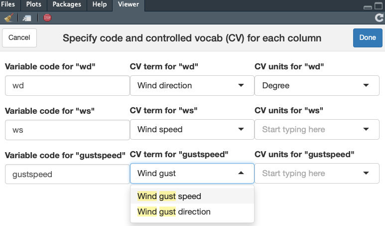
The type of data in each column needs to be described in a "variables list" with terms and units from a controlled vocabulary. Create this list for a dataset using a shiny gadget (opens in the Viewer pane of RStudio) with the function make_vars_list().

vars_list <- make_vars_list(ts_data)

vars_list <- list(
  'wd' = list(
    column = 'wd', 
    name = 'Wind direction', 
    units = 'Degree'),
  'ws' = list(
    column = 'ws', 
    name = 'Wind speed', 
    units = 'Meter per Second'),
  'gustspeed' = list(
    column = 'gustspeed', 
    name = 'Wind gust speed', 
    units = 'Meter per Second')
)

Once the vars_list is created, use it in the db_insert_results_ts() function to upload data along with its associated metadata

db_insert_results_ts(db, 
                     datavalues = ts_data,
                     methodcode = "SA",
                     site_code = "501R1",
                     variables = vars_list,
                     sampledmedium = "air")

Data associated with samples taken in the field and a property measured in the lab needs to have at least 4 columns corresponding to Timestamp, Site ID, Sample ID, and data value.

sample_data <- tibble::tibble(Timestamp = c("2018-06-27 13:45:00", "2018-07-27 13:55:00"),
                              Site = c("501R1", "501R1"),
                              Sample = c("DOC001", "DOC002"),
                              DOC = c(10, 12.3))
knitr::kable(sample_data)

Sample data are inserted with db_insert_results_samples() which requires metadata about both the method used to collect samples as well as the method used to analyze the sample. Provide details using db_describe_%METADATA%() functions.

db_describe_method(db, methodname = "Shimadzu", 
                   methodtypecv = "specimenAnalysis",
                   methodcode = "Shimadzu")
db_describe_method(db, methodname = "Water sample", 
                   methodtypecv = "specimenCollection",
                   methodcode = "watersamp")

vars_list <- make_vars_list(sample_data)

vars_list <- list(
  'DOC' = list(
    column = 'DOC', 
    name = 'Carbon, dissolved organic', 
    units = 'Milligram per Liter')
)

db_insert_results_samples(db, 
                          sample_data, 
                          field_method = "watersamp",
                          lab_method = "Shimadzu", 
                          variables = vars_list, 
                          sampledmedium = "liquidAqueous")

The insert function assumes that Site IDs are in a column called "Site" and Sample IDs are in a column called "Sample" but you can specify otherwise with the arguments site_code_col and sample_code_col. See more options for specifying metadata in the documentation for db_insert_results_samples()

4. Query

db_get_results() returns a list of dataframes with each type of result requested. By default retrieves data associated with all site codes and variables.

results_data <- db_get_results(db, result_type = c("ts", "sample"))
str(results_data)

Use list subsetting to get a data frame with time series (ts) results.

ts_data <- results_data[["Time_series_data"]]
# OR
ts_data <- results_data$Time_series_data

head(ts_data)

RSQLite::dbDisconnect(db)

More details

rodm2 is being designed to work either with an existing ODM2 database on a server (e.g. PostgreSQL), or with spreadsheet files that aren't (yet!) in a relational database. This package is intended to help populate, query, and visualize data that is organized with the ODM2 structure. It should not be necessary to understand ODM2 or SQL but it may help! See here for an overview of the data structure.

Acknowledgements

This project is made possible through support from rOpenSci and SESYNC.

Read about the details and development of ODM2 in the open access paper in Environmental Modelling & Software:

Horsburgh, J. S., Aufdenkampe, A. K., Mayorga, E., Lehnert, K. A., Hsu, L., Song, L., Spackman Jones, A., Damiano, S. G., Tarboton, D. G., Valentine, D., Zaslavsky, I., Whitenack, T. (2016). Observations Data Model 2: A community information model for spatially discrete Earth observations, Environmental Modelling & Software, 79, 55-74, http://dx.doi.org/10.1016/j.envsoft.2016.01.010

khondula/rodm2 documentation built on Jan. 9, 2020, 1:48 p.m.