README.md
In liangyy/silver-standard-performance: Generating PR/ROC curves in light and flexible way
silver-standard-performance
Overview
SilverStandardPerformance is an light-weight R package.
Its main functionality is to evaluate the performance of gene prioritization methods for complex traits, e.g. coloc, PrediXcan, smr, enloc, etc.
The evaluation simply relies on an external "ground truth" and the performance is simply how well the method can prioritize the "ground truth" trait/gene pairs relative to other trait/gene pairs.
In other word, we simply frame the evaluation problem as a typical problem for evaluating the performance of a binary classifier.
The only difference is that we don't have the ideal "ground truth".
Instead, we build several "silver standard"s as the imperfect surrogate of "ground truth".
Rationales behind the silver standard
For the purpose of evaluating how well the method prioritizes causal genes for complex traits, the ideal "silver standard" should list the (likely) causal genes for each of the complex traits.
An additional requirement for the "silver standard" is that it should be independent (apparently it is hard to achieve) to GWAS since many of the prioritization methods make use of GWAS results.
Following this rationale, we composed a rare variant association based silver standard which included height and lipid traits (LDL, HDL, TG, and high cholesterol), which can be loaded by typing
> data("rare_variant_based_silver_standard")
in R console.
However, as you may notice, this silver standard is very limited in terms of the number of both traits and genes being included.
Also, the result is still association-based rather than causality and many of the included trait/gene pairs are lack of experimental validation.
In fact, the gene-to-complex-trait information is currently very sparse (and that's why we care about the prioritization of causal genes for complex traits).
On the other hand, there are databases for causal genes of Mendelian diseases and rare diseases.
Since these phenotypes are mostly monogenic/oligogenic, the causal gene to phenotype mapping is of high confidence.
To make use of these great resources, we make extra hypothesis that:
The causal genes of the monogenic/oligogenic rare/Mendelian diseases can have milder effect on the relevant complex traits. So, if we can find the 'relevant' complex traits for these rare/Mendelian diseases, we can build another trait/gene silver standard by extrapolating to complex trait.
In this case, the big effect (due to deletion or coding variation) in rare/Mendelian diseases is extrapolate to the mild effect (probably via non-coding variation) in the relevant complex trait (see GTEx GWAS paper for more discussion on this topic).
To do so, we mapped complex traits to rare/Mendelian phenotypes with the use of phenotype ontology.
For complex trait phenotypes, we use
- EFO paper website. Comment: As used in GWAS Catalog. It describes quantitative traits, like height.
- HPO paper website. Comment: It mostly describes human abnormal phenotypes.
- phecode paper website. Comment: it is derived from ICD code.
Besides, the map among EFO, HPO, and phecode terms is achievable.
Phecode has been mapped to HPO (see this paper for more details).
Phecode has also been mapped to GWAS Catalog traits (see this paper for more details) which are further mapped to EFO terms.
For establishing the map between complex traits and rare/Mendelian phenotypes, HPO provides annotations to rare/Mendelian databases such as OMIM and Orphanet.
Using all of these resources, we obtained maps among HPO, phecode, and MIM/Orphanet phenotypes and Orphanet to gene map which were curated and provided by Lisa Bastarache (great thanks!).
We then went through some extra steps like formatting and mapping MIM phenotypes to MIM genes (information on the related scripts are at here).
These gave rise to the OMIM based silver standard and Orphanet based silver standard.
You can load these two datasets by typing
> data("omim_based_silver_standard")
> data("orphanet_based_silver_standard")
As you may notice, these silver standards are far from perfect.
We should use and interpret the results with cautious while keeping in mind the imperfectness and potential bias of the silver standard.
For your reference, we discuss some of the limitations of the current silver standard at here.
Get started
Suppose you have prioritization scores being calculated for each of the trait/gene pairs transcriptome-wide, you are ready to use SilverStandardPerformance to evaluate the performance of the prioritization using the silver standard provided along with the package.
And furthermore, if you have multiple scoring schemes to compare, you can include them all at once.
The followings are some extra but easy steps you need to take before getting ROC and PR curves done.
Step 1: Prepare/format your score table.
| trait | gene | predixcan_score | enloc_score |
|:-----------------------------------------:|:---------------:|:---------------:|:-----------:|
| UKB_20002_1466_self_reported_gout | ENSG00000112763 | 3.665 | 0 |
| Astle_et_al_2016_Lymphocyte_counts | ENSG00000223953 | 1.411 | 0.017 |
| UKB_20002_1065_self_reported_hypertension | ENSG00000213722 | 9.81 | 0.169 |
| Astle_et_al_2016_White_blood_cell_count | ENSG00000109066 | 3.12 | 0.012 |
| UKB_20002_1111_self_reported_asthma | ENSG00000149485 | 10.36 | 0.676 |
Comment: it should be a data.frame in R with one column named as 'trait' and one column named as 'gene'. The additional columns are interpreted as columns for different scoring schemes. Besides, the gene name should be Ensembl ID (without dot) and we may allow other gene names in the future.
Step 2: Prepare a map table mapping your traits to EFO, HPO, or phecode.
| trait | phecode | HPO |
|:-----------------------------------------:|:-------:|:-----------:|
| CARDIoGRAM_C4D_CAD_ADDITIVE | 411.4 | HP:0003362 |
| UKB_G43_Diagnoses_main_ICD10_G43_Migraine | 340.1 | HP:0002083 |
| UKB_20002_1309_self_reported_osteoporosis | 743 | HP:0006462 |
| EGG_BMI_HapMapImputed | 278.1 | HP:0012743 |
| GLGC_Mc_TG | 272.12 | HP:0003362 |
To assign one of the ontolog code to your trait makes the software "understand" what your trait really is.
To obtain the ontolog code for your trait, you can go to HPO, EFO (GWAS Catalog website may also work), and phecode websites listed above and search for the relevant terms.
As a tip, for disease phenotypes, HPO and phecode best suit the purpose and for non-disease quantitative traits, EFO may work better.
Comment: you can add another column named 'EFO' if you want to include EFO terms and it should be in the form like 'EFO:0004339'.
Step 3 (optional): Prepare a list of GWAS loci you care about.
If you want to limit the analysis to GWAS loci which overlaps silver standard genes and candidate genes nearby such GWAS loci, you need to specify the list of GWAS loci as follow.
| chromosome | start | end | trait | panel_variant_id |
|:----------:|:---------:|:---------:|:----------------------:|:-----------------------:|
| chr12 | 12580594 | 15088550 | UKB_50_Standing_height | chr12_14485920_C_T_b38 |
| chr10 | 102620653 | 104935290 | UKB_50_Standing_height | chr10_102764890_G_A_b38 |
| chr7 | 25869935 | 28320690 | UKB_50_Standing_height | chr7_25884464_T_C_b38 |
| chr11 | 46984586 | 49844498 | GLGC_Mc_HDL | chr11_48628939_T_C_b38 |
| chr18 | 48413361 | 50204214 | UKB_50_Standing_height | chr18_49200370_G_A_b38 |
Comment: the required columns are 'chromosome', 'start', 'end', and 'trait'. The additional columns won't be used. More importantly, the genomic position should be in hg38 (at least its version should match the other input, gene annotation, but currently we only provide gene annotation in hg38).
Note that we do recommend user to enable this pre-processing step in the analysis thanks to the imperfectness of the silver standard.
For more information, you can take a look at the discussion here and here.
Additional note for Step 3: Convert GWAS variant to GWAS locus.
For user who has the list of GWAS leading variants, we provide a utility function to extract the LD blocks containing the GWAS variants as the list of GWAS loci.
Note that, currently we only have LD block annotations for Europeans (by Berisa et al) so please use with cautious.
To do so, you should first format your GWAS variants as follow:
| chromosome | position | trait | panel_variant_id |
|:----------:|:---------:|:----------------------:|:-----------------------:|
| chr17 | 40430932 | UKB_50_Standing_height | chr17_40430932_A_G_b38 |
| chr2 | 199592665 | UKB_50_Standing_height | chr2_199592665_C_A_b38 |
| chr2 | 2.1e+07 | GLGC_Mc_LDL | chr2_21000700_G_A_b38 |
| chr12 | 102432745 | UKB_50_Standing_height | chr12_102432745_G_A_b38 |
| chr2 | 219129545 | UKB_50_Standing_height | chr2_219129545_G_A_b38 |
Comment: it should have columns named 'chromosome', 'position', and 'trait' at the minimal. Additional columns won't be used.
Suppose the above table is loaded as data.frame in R console with variable name gwas_variants, you can obtain GWAS loci (defined by LD block) by typing
> data("ld_block_pickrell_eur_b38")
> gwas_loci = SilverStandardPerformance:::gwas_hit_to_gwas_loci_by_ld_block(
    gwas_hit = gwas_variants,
    ld_block = ld_block_pickrell_eur_b38
  )
Comments: ld_block_pickrell_eur_b38 is the dataset of European LD blocks reported by Berisa et al in hg38. The input gwas_variants should use the same version to indicate the genomic position.
The above command gives rise to the following data.frame in gwas_loci.
| chromosome | position | trait | panel_variant_id | region_name | start | end |
|:----------:|:---------:|:----------------------:|:-----------------------:|:-----------:|:---------:|:---------:|
| chr17 | 40430932 | UKB_50_Standing_height | chr17_40430932_A_G_b38 | chr17_23 | 38653091 | 40721152 |
| chr2 | 199592665 | UKB_50_Standing_height | chr2_199592665_C_A_b38 | chr2_118 | 198446401 | 200711561 |
| chr2 | 2.1e+07 | GLGC_Mc_LDL | chr2_21000700_G_A_b38 | chr2_13 | 20850730 | 23118512 |
| chr12 | 102432745 | UKB_50_Standing_height | chr12_102432745_G_A_b38 | chr12_61 | 101468912 | 102571208 |
| chr2 | 219129545 | UKB_50_Standing_height | chr2_219129545_G_A_b38 | chr2_129 | 217530757 | 219589829 |
, where the additional three columns (at the very right) are the annotated LD blocks for each GWAS variant which can be used as GWAS loci for downstream analysis.
Step 4: Perform the actual analysis
Once you prepared the data.frame containing scores (e.g. score_table) and the data.frame mapping trait to phenotype ontology (e.g. map_table), it is time to perform the actual analysis using function silver_standard_perf.
Before running, you need to select a silver standard.
To see what silver standard datasets are available, you can type
> data(package = 'SilverStandardPerformance')
in R console.
The ones named as *_silver_standard are the available silver standards.
Suppose omim_based_silver_standard is selected to run the analysis, then all you need to do is:
> data("omim_based_silver_standard")
> output = silver_standard_perf(
    score_table = score_table,
    map_table = map_table,
    silver_standard = omim_based_silver_standard,
    # suppose you want to map the your traits to silver standard phenotypes using
    # both 'HPO' and 'phecode' (the order does not matter)
    trait_codes = c('HPO', 'phecode')
  )
If you want to limit the analysis to a list of GWAS loci (see why you may want to do this here and here),
then you can do:
> data("omim_based_silver_standard")
> # load gene annotation file provided along with the package, which tells the location of each gene
> data("gene_annotation_gencode_v26_hg38")
> output = silver_standard_perf(
    score_table = score_table,
    map_table = map_table,
    silver_standard = omim_based_silver_standard,
    trait_codes = c('HPO', 'phecode'),
    ##### the additional two inputs required #####
    # 1. data.frame where each row is a GWAS locus of a trait.
    # The genome assembly version should match gene_annotation
    gwas_loci = gwas_loci,
    # 2. data.frame of gene annotation provided as a dataset in SilverStandardPerformance
    gene_annotation = gene_annotation_gencode_v26_hg38$gene_annotation
  )
The output contains PR curves and ROC curves as two ggplot objects along with ROC AUCs, see example.
Additional note on limiting analysis to GWAS loci
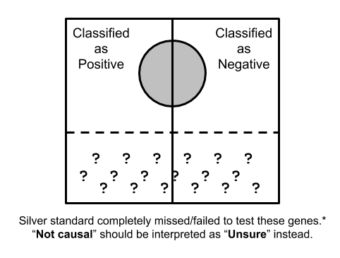
Suppose the whole quadrangle represents the all possible trait/gene pairs, and the silver circle in the middle represents the set of trait/gene pairs that are considered as 'causal' in a silver standard.
The vertical line in the middle is showing how a classifier would split the trait/gene pairs into "positive" and "negative" instances according to a scoring scheme along with the score cutoff.
However, as we discussed here, silver standard is imperfect and it contains false positives and more importantly a huge amount of false negatives.
For instance, many genes with milder effect won't cause monogenic disease so that OMIM-based silver standard will completely miss them.
As another example, if the effect of a gene is mostly via regulatory mechanism or it does not have enough coding variation, it won't be implicated in rare variant-based studies due to un-matched molecular mechanism or lack of statistical power.
In other word, there are many causal genes in complex traits that are completely missed in current silver standard datasets.
To account for this fact, we suggest to limit the analysis to trait/gene pairs nearby silver standard.
Here, we make the additional assumption that: Silver standard trait/gene pair is the only causal one within the locus.
In other word, the silver standard trait/gene pair can completely explain the GWAS signal of the locus.
For trait/gene pairs far from any silver standard, we consider their statuses as "unknown" rather than "not causal", and these instances correspond to the quadrangle labelled with question marks in the figure.
Following this idea, we recommend people to limit the analysis to GWAS loci containing silver standard genes for two reasons:
- The original goal is to prioritize gene for GWAS hits (we care about interpreting signals rather than interpreting anything);
- We should exclude GWAS loci without silver standard genes since the silver standard is really unsure about these regions.
liangyy/silver-standard-performance documentation built on Dec. 5, 2019, 8:53 a.m.
R Package Documentation
Browse R Packages
We want your feedback!
Note that we can't provide technical support on individual packages. You should contact the package authors for that.
silver-standard-performance
Overview
SilverStandardPerformance is an light-weight R package. Its main functionality is to evaluate the performance of gene prioritization methods for complex traits, e.g. coloc, PrediXcan, smr, enloc, etc. The evaluation simply relies on an external "ground truth" and the performance is simply how well the method can prioritize the "ground truth" trait/gene pairs relative to other trait/gene pairs. In other word, we simply frame the evaluation problem as a typical problem for evaluating the performance of a binary classifier. The only difference is that we don't have the ideal "ground truth". Instead, we build several "silver standard"s as the imperfect surrogate of "ground truth".
Rationales behind the silver standard
For the purpose of evaluating how well the method prioritizes causal genes for complex traits, the ideal "silver standard" should list the (likely) causal genes for each of the complex traits. An additional requirement for the "silver standard" is that it should be independent (apparently it is hard to achieve) to GWAS since many of the prioritization methods make use of GWAS results.
Following this rationale, we composed a rare variant association based silver standard which included height and lipid traits (LDL, HDL, TG, and high cholesterol), which can be loaded by typing
> data("rare_variant_based_silver_standard")
in R console. However, as you may notice, this silver standard is very limited in terms of the number of both traits and genes being included. Also, the result is still association-based rather than causality and many of the included trait/gene pairs are lack of experimental validation. In fact, the gene-to-complex-trait information is currently very sparse (and that's why we care about the prioritization of causal genes for complex traits).
On the other hand, there are databases for causal genes of Mendelian diseases and rare diseases. Since these phenotypes are mostly monogenic/oligogenic, the causal gene to phenotype mapping is of high confidence. To make use of these great resources, we make extra hypothesis that: The causal genes of the monogenic/oligogenic rare/Mendelian diseases can have milder effect on the relevant complex traits. So, if we can find the 'relevant' complex traits for these rare/Mendelian diseases, we can build another trait/gene silver standard by extrapolating to complex trait. In this case, the big effect (due to deletion or coding variation) in rare/Mendelian diseases is extrapolate to the mild effect (probably via non-coding variation) in the relevant complex trait (see GTEx GWAS paper for more discussion on this topic).
To do so, we mapped complex traits to rare/Mendelian phenotypes with the use of phenotype ontology. For complex trait phenotypes, we use
- EFO paper website. Comment: As used in GWAS Catalog. It describes quantitative traits, like height.
- HPO paper website. Comment: It mostly describes human abnormal phenotypes.
- phecode paper website. Comment: it is derived from ICD code.
Besides, the map among EFO, HPO, and phecode terms is achievable. Phecode has been mapped to HPO (see this paper for more details). Phecode has also been mapped to GWAS Catalog traits (see this paper for more details) which are further mapped to EFO terms.
For establishing the map between complex traits and rare/Mendelian phenotypes, HPO provides annotations to rare/Mendelian databases such as OMIM and Orphanet. Using all of these resources, we obtained maps among HPO, phecode, and MIM/Orphanet phenotypes and Orphanet to gene map which were curated and provided by Lisa Bastarache (great thanks!). We then went through some extra steps like formatting and mapping MIM phenotypes to MIM genes (information on the related scripts are at here). These gave rise to the OMIM based silver standard and Orphanet based silver standard. You can load these two datasets by typing
> data("omim_based_silver_standard")
> data("orphanet_based_silver_standard")
As you may notice, these silver standards are far from perfect. We should use and interpret the results with cautious while keeping in mind the imperfectness and potential bias of the silver standard. For your reference, we discuss some of the limitations of the current silver standard at here.
Get started
Suppose you have prioritization scores being calculated for each of the trait/gene pairs transcriptome-wide, you are ready to use SilverStandardPerformance to evaluate the performance of the prioritization using the silver standard provided along with the package.
And furthermore, if you have multiple scoring schemes to compare, you can include them all at once.
The followings are some extra but easy steps you need to take before getting ROC and PR curves done.
Step 1: Prepare/format your score table.
| trait | gene | predixcan_score | enloc_score | |:-----------------------------------------:|:---------------:|:---------------:|:-----------:| | UKB_20002_1466_self_reported_gout | ENSG00000112763 | 3.665 | 0 | | Astle_et_al_2016_Lymphocyte_counts | ENSG00000223953 | 1.411 | 0.017 | | UKB_20002_1065_self_reported_hypertension | ENSG00000213722 | 9.81 | 0.169 | | Astle_et_al_2016_White_blood_cell_count | ENSG00000109066 | 3.12 | 0.012 | | UKB_20002_1111_self_reported_asthma | ENSG00000149485 | 10.36 | 0.676 |
Comment: it should be a data.frame in R with one column named as 'trait' and one column named as 'gene'. The additional columns are interpreted as columns for different scoring schemes. Besides, the gene name should be Ensembl ID (without dot) and we may allow other gene names in the future.
Step 2: Prepare a map table mapping your traits to EFO, HPO, or phecode.
| trait | phecode | HPO | |:-----------------------------------------:|:-------:|:-----------:| | CARDIoGRAM_C4D_CAD_ADDITIVE | 411.4 | HP:0003362 | | UKB_G43_Diagnoses_main_ICD10_G43_Migraine | 340.1 | HP:0002083 | | UKB_20002_1309_self_reported_osteoporosis | 743 | HP:0006462 | | EGG_BMI_HapMapImputed | 278.1 | HP:0012743 | | GLGC_Mc_TG | 272.12 | HP:0003362 |
To assign one of the ontolog code to your trait makes the software "understand" what your trait really is. To obtain the ontolog code for your trait, you can go to HPO, EFO (GWAS Catalog website may also work), and phecode websites listed above and search for the relevant terms. As a tip, for disease phenotypes, HPO and phecode best suit the purpose and for non-disease quantitative traits, EFO may work better.
Comment: you can add another column named 'EFO' if you want to include EFO terms and it should be in the form like 'EFO:0004339'.
Step 3 (optional): Prepare a list of GWAS loci you care about.
If you want to limit the analysis to GWAS loci which overlaps silver standard genes and candidate genes nearby such GWAS loci, you need to specify the list of GWAS loci as follow.
| chromosome | start | end | trait | panel_variant_id | |:----------:|:---------:|:---------:|:----------------------:|:-----------------------:| | chr12 | 12580594 | 15088550 | UKB_50_Standing_height | chr12_14485920_C_T_b38 | | chr10 | 102620653 | 104935290 | UKB_50_Standing_height | chr10_102764890_G_A_b38 | | chr7 | 25869935 | 28320690 | UKB_50_Standing_height | chr7_25884464_T_C_b38 | | chr11 | 46984586 | 49844498 | GLGC_Mc_HDL | chr11_48628939_T_C_b38 | | chr18 | 48413361 | 50204214 | UKB_50_Standing_height | chr18_49200370_G_A_b38 |
Comment: the required columns are 'chromosome', 'start', 'end', and 'trait'. The additional columns won't be used. More importantly, the genomic position should be in hg38 (at least its version should match the other input, gene annotation, but currently we only provide gene annotation in hg38).
Note that we do recommend user to enable this pre-processing step in the analysis thanks to the imperfectness of the silver standard. For more information, you can take a look at the discussion here and here.
Additional note for Step 3: Convert GWAS variant to GWAS locus.
For user who has the list of GWAS leading variants, we provide a utility function to extract the LD blocks containing the GWAS variants as the list of GWAS loci. Note that, currently we only have LD block annotations for Europeans (by Berisa et al) so please use with cautious.
To do so, you should first format your GWAS variants as follow:
| chromosome | position | trait | panel_variant_id | |:----------:|:---------:|:----------------------:|:-----------------------:| | chr17 | 40430932 | UKB_50_Standing_height | chr17_40430932_A_G_b38 | | chr2 | 199592665 | UKB_50_Standing_height | chr2_199592665_C_A_b38 | | chr2 | 2.1e+07 | GLGC_Mc_LDL | chr2_21000700_G_A_b38 | | chr12 | 102432745 | UKB_50_Standing_height | chr12_102432745_G_A_b38 | | chr2 | 219129545 | UKB_50_Standing_height | chr2_219129545_G_A_b38 |
Comment: it should have columns named 'chromosome', 'position', and 'trait' at the minimal. Additional columns won't be used.
Suppose the above table is loaded as data.frame in R console with variable name gwas_variants, you can obtain GWAS loci (defined by LD block) by typing
> data("ld_block_pickrell_eur_b38")
> gwas_loci = SilverStandardPerformance:::gwas_hit_to_gwas_loci_by_ld_block(
gwas_hit = gwas_variants,
ld_block = ld_block_pickrell_eur_b38
)
Comments: ld_block_pickrell_eur_b38 is the dataset of European LD blocks reported by Berisa et al in hg38. The input gwas_variants should use the same version to indicate the genomic position.
The above command gives rise to the following data.frame in gwas_loci.
| chromosome | position | trait | panel_variant_id | region_name | start | end | |:----------:|:---------:|:----------------------:|:-----------------------:|:-----------:|:---------:|:---------:| | chr17 | 40430932 | UKB_50_Standing_height | chr17_40430932_A_G_b38 | chr17_23 | 38653091 | 40721152 | | chr2 | 199592665 | UKB_50_Standing_height | chr2_199592665_C_A_b38 | chr2_118 | 198446401 | 200711561 | | chr2 | 2.1e+07 | GLGC_Mc_LDL | chr2_21000700_G_A_b38 | chr2_13 | 20850730 | 23118512 | | chr12 | 102432745 | UKB_50_Standing_height | chr12_102432745_G_A_b38 | chr12_61 | 101468912 | 102571208 | | chr2 | 219129545 | UKB_50_Standing_height | chr2_219129545_G_A_b38 | chr2_129 | 217530757 | 219589829 |
, where the additional three columns (at the very right) are the annotated LD blocks for each GWAS variant which can be used as GWAS loci for downstream analysis.
Step 4: Perform the actual analysis
Once you prepared the data.frame containing scores (e.g. score_table) and the data.frame mapping trait to phenotype ontology (e.g. map_table), it is time to perform the actual analysis using function silver_standard_perf.
Before running, you need to select a silver standard. To see what silver standard datasets are available, you can type
> data(package = 'SilverStandardPerformance')
in R console.
The ones named as *_silver_standard are the available silver standards.
Suppose omim_based_silver_standard is selected to run the analysis, then all you need to do is:
> data("omim_based_silver_standard")
> output = silver_standard_perf(
score_table = score_table,
map_table = map_table,
silver_standard = omim_based_silver_standard,
# suppose you want to map the your traits to silver standard phenotypes using
# both 'HPO' and 'phecode' (the order does not matter)
trait_codes = c('HPO', 'phecode')
)
If you want to limit the analysis to a list of GWAS loci (see why you may want to do this here and here), then you can do:
> data("omim_based_silver_standard")
> # load gene annotation file provided along with the package, which tells the location of each gene
> data("gene_annotation_gencode_v26_hg38")
> output = silver_standard_perf(
score_table = score_table,
map_table = map_table,
silver_standard = omim_based_silver_standard,
trait_codes = c('HPO', 'phecode'),
##### the additional two inputs required #####
# 1. data.frame where each row is a GWAS locus of a trait.
# The genome assembly version should match gene_annotation
gwas_loci = gwas_loci,
# 2. data.frame of gene annotation provided as a dataset in SilverStandardPerformance
gene_annotation = gene_annotation_gencode_v26_hg38$gene_annotation
)
The output contains PR curves and ROC curves as two ggplot objects along with ROC AUCs, see example.
Additional note on limiting analysis to GWAS loci
Suppose the whole quadrangle represents the all possible trait/gene pairs, and the silver circle in the middle represents the set of trait/gene pairs that are considered as 'causal' in a silver standard. The vertical line in the middle is showing how a classifier would split the trait/gene pairs into "positive" and "negative" instances according to a scoring scheme along with the score cutoff.
However, as we discussed here, silver standard is imperfect and it contains false positives and more importantly a huge amount of false negatives. For instance, many genes with milder effect won't cause monogenic disease so that OMIM-based silver standard will completely miss them. As another example, if the effect of a gene is mostly via regulatory mechanism or it does not have enough coding variation, it won't be implicated in rare variant-based studies due to un-matched molecular mechanism or lack of statistical power. In other word, there are many causal genes in complex traits that are completely missed in current silver standard datasets.
To account for this fact, we suggest to limit the analysis to trait/gene pairs nearby silver standard. Here, we make the additional assumption that: Silver standard trait/gene pair is the only causal one within the locus. In other word, the silver standard trait/gene pair can completely explain the GWAS signal of the locus. For trait/gene pairs far from any silver standard, we consider their statuses as "unknown" rather than "not causal", and these instances correspond to the quadrangle labelled with question marks in the figure.
Following this idea, we recommend people to limit the analysis to GWAS loci containing silver standard genes for two reasons:
- The original goal is to prioritize gene for GWAS hits (we care about interpreting signals rather than interpreting anything);
- We should exclude GWAS loci without silver standard genes since the silver standard is really unsure about these regions.
R Package Documentation
Browse R Packages
We want your feedback!
Note that we can't provide technical support on individual packages. You should contact the package authors for that.
Embedding an R snippet on your website
Add the following code to your website.
For more information on customizing the embed code, read Embedding Snippets.