In timjmiller/wham: Woods Hole Assessment Model (WHAM)
knitr::opts_chunk$set(
  collapse = TRUE,
  comment = "#>"
)
wham.dir <- find.package("wham")
knitr::opts_knit$set(root.dir = file.path(wham.dir,"extdata"))
library(knitr)
library(kableExtra)
In this vignette we walk through an example using the wham (WHAM = Woods Hole Assessment Model) package to run a state-space age-structured stock assessment model. WHAM is a generalization of code written for Miller et al. (2016) and Xu et al. (2018), and in this example we apply WHAM to the same stock, Southern New England / Mid-Atlantic Yellowtail Flounder.
This is the 5th WHAM example, which builds off example 2:
- full state-space model (numbers-at-age are random effects for all ages,
NAA_re = list(sigma='rec+1',cor='iid'))
- logistic normal age compositions, pooling zero observations with adjacent ages (
age_comp = "logistic-normal-pool0")
- random-about-mean recruitment (
recruit_model = 2)
- 5 indices
- fit to 1973-2011 data
We assume you already have wham installed. If not, see the Introduction. The simpler 1st example, without environmental effects or time-varying $M$, is available as a R script and vignette.
In example 5, we demonstrate how to specify and run WHAM with the following options for natural mortality:
- not estimated (fixed at input values)
- one value, $M$
- age-specific, $M_a$ (independent)
- function of weight-at-age, $M_{y,a} = \mu_M * W_{y,a}^b$
- AR1 deviations by age (random effects), $M_{y,a} = \mu_M + \delta_a \quad\mathrm{and}\quad \delta_a \sim \mathcal{N} (\rho_a \delta_{a-1}, \sigma^2_M)$
- AR1 deviations by year (random effects), $M_{y,a} = \mu_M + \delta_y \quad\mathrm{and}\quad \delta_y \sim \mathcal{N} (\rho_y \delta_{y-1}, \sigma^2_M)$
- 2D AR1 deviations by age and year (random effects), $M_{y,a} = M_a + \delta_{y,a} \quad\mathrm{and}\quad \delta_{y,a} \sim \mathcal{N}(0,\Sigma)$
We also demonstrate alternate specifications for the link between $M$ and an environmental covariate, the Gulf Stream Index (GSI), as in O'Leary et al. (2019):
- none
- linear (in log-space), $M_{y,a} = e^{\mathrm{log}\mu_M + \beta_1 E_y}$
- quadratic (in log-space), $M_{y,a} = e^{\mathrm{log}\mu_M + \beta_1 E_y + \beta_2 E^2_y}$
Note that you can specify more than one of the above effects on $M$, although the model may not be estimable. For example, the most complex model with weight-at-age, 2D AR1 age- and year-deviations, and a quadratic environmental effect: $M_{y,a} = e^{\mathrm{log}\mu_M + b W_{y,a} + \beta_1 E_y + \beta_2 E^2_y + \delta_{y,a}}$.
1. Load data
Open R and load the wham package:
library(wham)
library(tidyverse)
library(viridis)
For a clean, runnable .R script, look at ex5_M_GSI.R in the example_scripts folder of the wham package install:
wham.dir <- find.package("wham")
file.path(wham.dir, "example_scripts")
You can run this entire example script with:
write.dir <- "choose/where/to/save/output" # otherwise will be saved in working directory
source(file.path(wham.dir, "example_scripts", "ex5_M_GSI.R"))
Let's create a directory for this analysis:
# choose a location to save output, otherwise will be saved in working directory
write.dir <- "choose/where/to/save/output"
dir.create(write.dir)
setwd(write.dir)
We need the same ASAP data file as in example 2, and the environmental covariate (GSI). Let's copy ex2_SNEMAYT.dat and GSI.csv to our analysis directory:
wham.dir <- find.package("wham")
file.copy(from=file.path(wham.dir,"extdata","ex2_SNEMAYT.dat"), to=write.dir, overwrite=FALSE)
file.copy(from=file.path(wham.dir,"extdata","GSI.csv"), to=write.dir, overwrite=FALSE)
Confirm you are in the correct directory and it has the required data files:
list.files()
Read the ASAP3 .dat file into R and convert to input list for wham:
asap3 <- read_asap3_dat("ex2_SNEMAYT.dat")
Load the environmental covariate (Gulf Stream Index, GSI) data into R:
env.dat <- read.csv("GSI.csv", header=T)
head(env.dat)
The GSI does not have a standard error estimate, either for each yearly observation or one overall value. In such a case, WHAM can estimate the observation error for the environmental covariate, either as one overall value, $\sigma_E$, or yearly values as random effects, $\mathrm{log}\sigma_{E_y} \sim \mathcal{N}(\mathrm{log}\sigma_E, \sigma^2_{\sigma_E})$. In this example we choose the simpler option and estimate one observation error parameter, shared across years.
2. Specify models
Now we specify several models with different options for natural mortality:
df.mods <- data.frame(M_model = c(rep("---",3),"age-specific","weight-at-age",rep("constant",5),"---"),
                      M_re = c(rep("none",6),"ar1_y","2dar1","none","none","2dar1"),
                      Ecov_process = rep("ar1",11),
                      Ecov_link = c(0,1,2,rep(0,5),1,2,0), stringsAsFactors=FALSE)
n.mods <- dim(df.mods)[1]
df.mods$Model <- paste0("m",1:n.mods)
df.mods <- df.mods %>% select(Model, everything()) # moves Model to first col
Look at the model table:
df.mods
3. Natural mortality options
Next we specify the options for modeling natural mortality by including an optional list argument, M, to the prepare_wham_input() function (see the prepare_wham_input() help page). M specifies estimation options and can overwrite M-at-age values specified in the ASAP data file. By default (i.e. M is NULL or not included), the M-at-age matrix from the ASAP data file is used (M fixed, not estimated). M is a list with the following entries:
-
$model: Natural mortality model options.
-
"constant": estimate a single $M$, shared across all ages and years.
"age-specific": estimate $M_a$ independent for each age, shared across years.-
"weight-at-age": estimate $M$ as a function of weight-at-age, $M_{y,a} = \mu_M * W_{y,a}^b$, as in Lorenzen (1996) and Miller & Hyun (2018).
-
$re: Time- and age-varying random effects on $M$.
-
"none": $M$ constant in time and across ages (default).
"iid": $M$ varies by year and age, but uncorrelated."ar1_a": $M$ correlated by age (AR1), constant in time."ar1_y": $M$ correlated by year (AR1), constant by age.-
"2dar1": $M$ correlated by year and age (2D AR1), as in Cadigan (2016).
-
$initial_means: Initial/mean M-at-age vector, with length = number of ages (if $model = "age-specific") or 1 (if $model = "weight-at-age" or "constant"). If NULL, initial mean M-at-age values are taken from the first row of the MAA matrix in the ASAP data file.
-
$est_ages: Vector of ages to estimate age-specific $M_a$ (others will be fixed at initial values). E.g. in a model with 6 ages, $est_ages = 5:6 will estimate $M_a$ for the 5th and 6th ages, and fix $M$ for ages 1-4. If NULL, $M$ at all ages is fixed at M$initial_means (if not NULL) or row 1 of the MAA matrix from the ASAP file (if M$initial_means = NULL).
-
$logb_prior: (Only for weight-at-age model) TRUE or FALSE (default), should a $\mathcal{N}(0.305, 0.08)$ prior be used on log_b? Based on Fig. 1 and Table 1 (marine fish) in Lorenzen (1996).
For example, to fit model m1, fix $M_a$ at values in ASAP file:
M <- NULL # or simply leave out of call to prepare_wham_input
To fit model m6, estimate one $M$, constant by year and age:
M <- list(model="constant", est_ages=1)
And to fit model m8, estimate mean $M$ with 2D AR1 deviations by year and age:
M <- list(model="constant", est_ages=1, re="2dar1")
To fit model m11, use the $M_a$ values specified in the ASAP file, but with 2D AR1 deviations as in Cadigan (2016):
M <- list(re="2dar1")
4. Linking M to an environmental covariate (GSI)
As described in example 2, the environmental covariate options are fed to prepare_wham_input() as a list, ecov. This example differs from example 2 in that:
$logsigma = "est_1": estimate the observation error for the GSI (one overall value for all years). The other option is "est_re" to allow the GSI observation error to have yearly fluctuations (random effects). The Cold Pool Index in example 2 had yearly observation errors given.$lag = 0: GSI in year t affects $M$ in year t, instead of year t+1.$where = "M": GSI affects $M$, instead of recruitment.$how: ecov$how = 0 estimates the GSI time-series model (AR1) for models without a GSI-M effect, in order to compare AIC with models that do include a GSI-M effect. Setting ecov$how = 1 is necessary to allow a GSI-M effect.$link_model: specifies the model linking GSI to $M$. Can be NA (no effect, default), "linear", or "poly-x" (where x is the degree of a polynomial). In this example we demonstrate models with no GSI-M effect, a linear GSI-M effect, and a quadratic GSI-M effect ("poly-2"). WHAM includes a function to calculate orthogonal polynomials in TMB, akin to the poly() function in R.
For example, the ecov list for model m3 with a quadratic GSI-M effect:
  # example for model m3
  ecov <- list(
    label = "GSI",
    mean = as.matrix(env.dat$GSI),
    logsigma = 'est_1', # estimate obs sigma, 1 value shared across years
    year = env.dat$year,
    use_obs = matrix(1, ncol=1, nrow=dim(env.dat)[1]), # use all obs (=1)
    lag = 0, # GSI in year t affects M in same year
    process_model = "ar1", # GSI modeled as AR1 (random walk would be "rw")
    where = "M", # GSI affects natural mortality
    how = 1, # include GSI effect on M
    link_model = "poly-2") # quadratic GSI-M effect
Note that you can set ecov = NULL to fit the model without environmental covariate data, but here we fit the ecov data even for models without GSI effect on $M$ (m1, m4-8) so that we can compare them via AIC (need to have the same data in the likelihood). We accomplish this by setting ecov$how = 0 and ecov$process_model = "ar1".
5. Run all models
All models use the same options for recruitment (random-about-mean, no stock-recruit function) and selectivity (logistic, with parameters fixed for indices 4 and 5).
env.dat <- read.csv("GSI.csv", header=T)
for(m in 1:n.mods){
  ecov <- list(
    label = "GSI",
    mean = as.matrix(env.dat$GSI),
    logsigma = 'est_1', # estimate obs sigma, 1 value shared across years
    year = env.dat$year,
    use_obs = matrix(1, ncol=1, nrow=dim(env.dat)[1]), # use all obs (=1)
    lag = 0, # GSI in year t affects M in same year
    process_model = df.mods$Ecov_process[m], # "rw" or "ar1"
    where = "M", # GSI affects natural mortality
    how = ifelse(df.mods$Ecov_link[m]==0,0,1), # 0 = no effect (but still fit Ecov to compare AIC), 1 = mean
    link_model = c(NA,"linear","poly-2")[df.mods$Ecov_link[m]+1])

  m_model <- df.mods$M_model[m]
  if(df.mods$M_model[m] == '---') m_model = "age-specific"
  if(df.mods$M_model[m] %in% c("constant","weight-at-age")) est_ages = 1
  if(df.mods$M_model[m] == "age-specific") est_ages = 1:asap3$dat$n_ages
  if(df.mods$M_model[m] == '---') est_ages = NULL

  M <- list(
    model = m_model,
    re = df.mods$M_re[m],
    est_ages = est_ages
  )
  if(m_model %in% c("constant","weight-at-age")) M$initial_means = 0.28

  input <- prepare_wham_input(asap3, recruit_model = 2,
                              model_name = paste0("m",m,": ", df.mods$M_model[m]," + ",c("no","linear","poly-2")[df.mods$Ecov_link[m]+1]," GSI link + ",df.mods$M_re[m]," devs"),
                              ecov = ecov,
                              selectivity=list(model=rep("logistic",6),
                                               initial_pars=c(rep(list(c(3,3)),4), list(c(1.5,0.1), c(1.5,0.1))),
                                               fix_pars=c(rep(list(NULL),4), list(1:2, 1:2))),
                              NAA_re = list(sigma='rec+1',cor='iid'),
                              M=M,
                              age_comp = "logistic-normal-pool0") # logistic normal pool 0 obs

  # Fit model
  mod <- fit_wham(input, do.retro=T, do.osa=F) # turn off OSA residuals to save time

  # Save model
  saveRDS(mod, file=paste0(df.mods$Model[m],".rds"))

  # If desired, plot output in new subfolder
  # plot_wham_output(mod=mod, dir.main=file.path(getwd(),df.mods$Model[m]), out.type='html')

  # If desired, do projections
  # mod_proj <- project_wham(mod)
  # saveRDS(mod_proj, file=paste0(df.mods$Model[m],"_proj.rds"))
}
6. Compare models
data(vign5_res)
# data(vign5_MAA)
Collect all models into a list.
mod.list <- paste0(df.mods$Model,".rds")
mods <- lapply(mod.list, readRDS)
Get model convergence and stats.
opt_conv = 1-sapply(mods, function(x) x$opt$convergence)
ok_sdrep = sapply(mods, function(x) if(x$na_sdrep==FALSE & !is.na(x$na_sdrep)) 1 else 0)
df.mods$conv <- as.logical(opt_conv)
df.mods$pdHess <- as.logical(ok_sdrep)
Only calculate AIC and Mohn's rho for converged models.
df.mods$runtime <- sapply(mods, function(x) x$runtime)
df.mods$NLL <- sapply(mods, function(x) round(x$opt$objective,3))
not_conv <- !df.mods$conv | !df.mods$pdHess
mods2 <- mods
mods2[not_conv] <- NULL
df.aic.tmp <- as.data.frame(compare_wham_models(mods2, sort=FALSE, calc.rho=T)$tab)
df.aic <- df.aic.tmp[FALSE,]
ct = 1
for(i in 1:n.mods){
  if(not_conv[i]){
    df.aic[i,] <- rep(NA,5)
  } else {
    df.aic[i,] <- df.aic.tmp[ct,]
    ct <- ct + 1
  }
}
df.aic[,1:2] <- format(round(df.aic[,1:2], 1), nsmall=1)
df.aic[,3:5] <- format(round(df.aic[,3:5], 3), nsmall=3)
df.aic[grep("NA",df.aic$dAIC),] <- "---"
df.mods <- cbind(df.mods, df.aic)
Make results table prettier.
df.mods$Ecov_link <- c("---","linear","poly-2")[df.mods$Ecov_link+1]
df.mods$M_re[df.mods$M_re=="none"] = "---"
colnames(df.mods)[2] = "M_est"
rownames(df.mods) <- NULL
Look at results table.
df.mods
7. Results
In the table, I have highlighted models which converged and successfully inverted the Hessian to produce SE estimates for all (fixed effect) parameters. WHAM stores this information in mod$na_sdrep (should be FALSE), mod$sdrep$pdHess (should be TRUE), and mod$opt$convergence (should be 0). See stats::nlminb() and TMB::sdreport() for details.
Models m8 (estimate mean $M$ and 2D AR1 deviations by year and age, no GSI effect) and m11 (keep mean $M$ fixed but estimate 2D AR1 deviations) had the lowest AIC and were overwhelmingly supported relative to the other models (bold in table below).
library(knitr)
library(kableExtra)
# vign5_res[,12:14] = round(vign5_res[,12:14], 3)
posdef = which(vign5_res$pdHess == TRUE)
thebest = c(8,11)
vign5_res %>%
  # mutate(na_sdrep = cell_spec(na_sdrep, "html", bold = ifelse(na_sdrep == TRUE,TRUE,FALSE))) %>%
  # select(everything()) %>%
  dplyr::rename("M model"="M_est", "GSI"="Ecov_process", "GSI link"="Ecov_link",
         "Converged"="conv", "Pos def\nHessian"="pdHess", "Runtime\n(min)"="runtime",
         "$\\rho_{R}$"="rho_R", "$\\rho_{SSB}$"="rho_SSB", "$\\rho_{\\overline{F}}$"="rho_Fbar") %>%
  kable(escape = F) %>%
  kable_styling(bootstrap_options = c("condensed","responsive")) %>%
  row_spec(posdef, background = gray.colors(10,end=0.95)[10]) %>%
  row_spec(thebest, bold=TRUE)
Estimated M
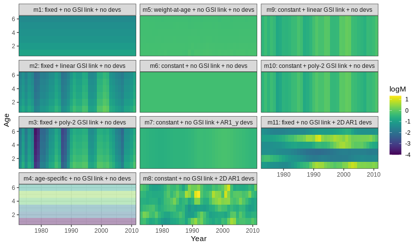
- Models allowed to estimate mean $M$ increased $M$ compared to the fixed values in
m1-3 (more green/yellow than blue).
- Models that estimated $M_a$ had highest $M_a$ for ages 4-5.
- Models that estimated $M_y$ had higher $M_y$ in the early 1990s and around 2000.
Below is a plot of $M$ by age (y-axis) and year (x-axis) for all models. Models with a positive definite Hessian are solid, and models with non-positive definite Hessian are pale.
 { width=90% }
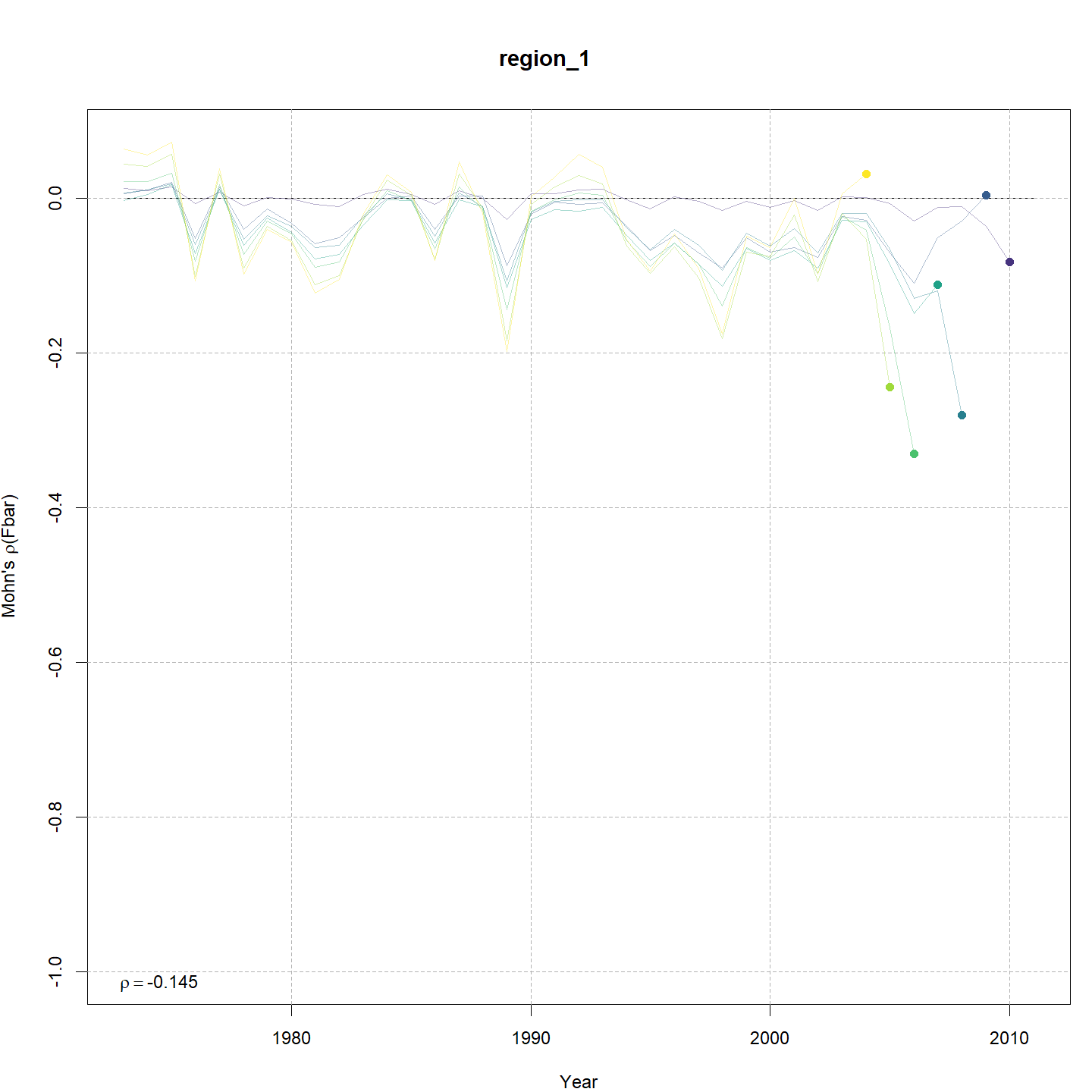
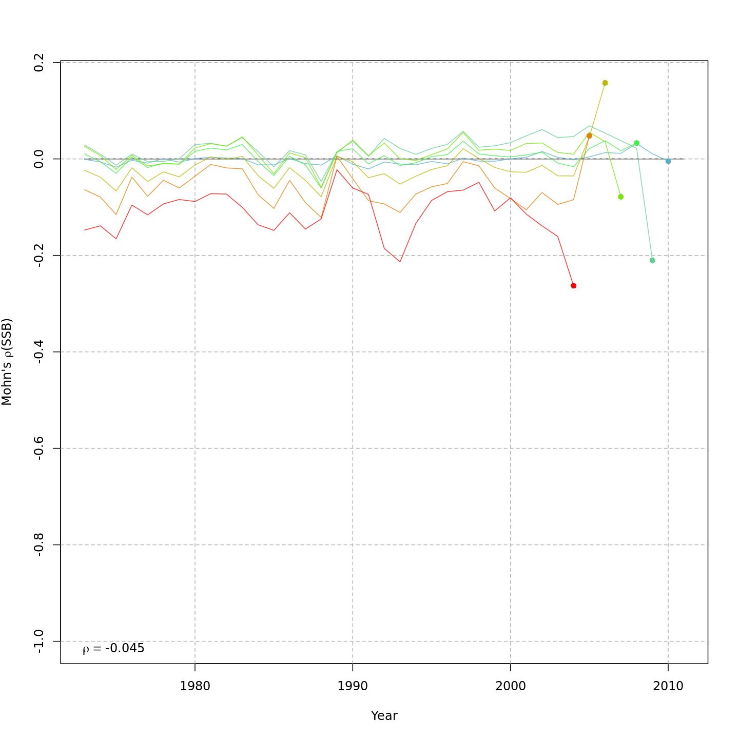
Retrospective patterns
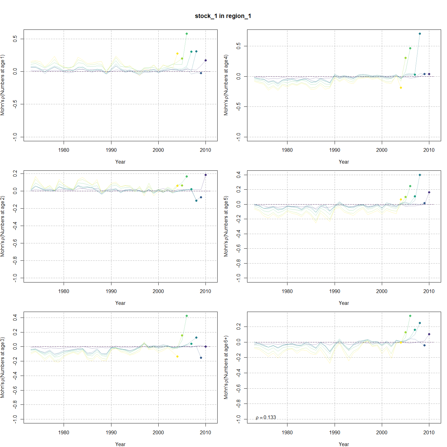
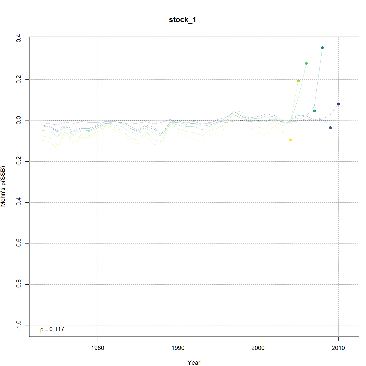
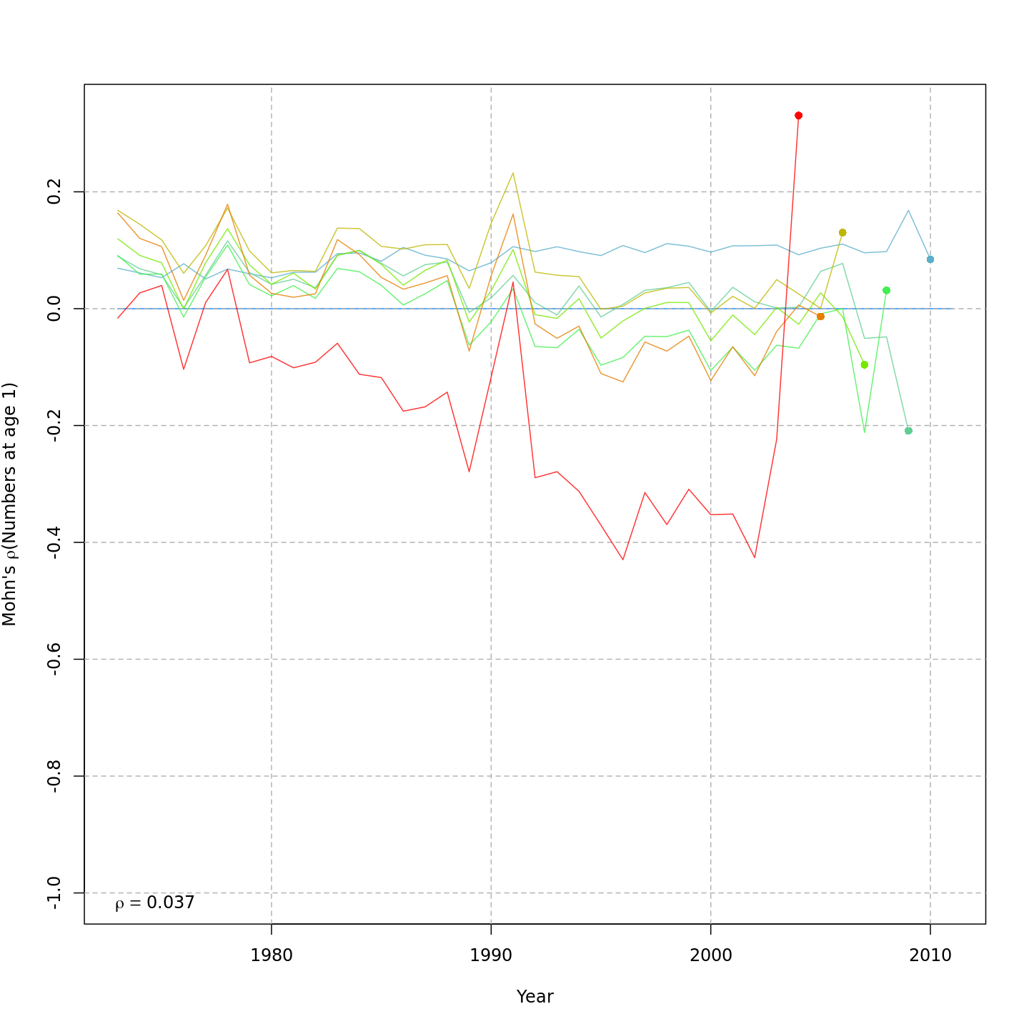
Compared to m1, the retrospective pattern for m8 was slightly worse for recruitment (m8 0.32, m1 0.23) but improved for SSB (m8 0.01, m1 0.07) and F (m8 -0.05, m1 -0.11). In general, models with GSI effects or 2D AR1 deviations on $M$ had reduced retrospective patterns compared to the status quo (m1) and models with 1D AR1 random effects on $M$. Compare the retrospective patterns of numbers-at-age, SSB, and F for models m1 (left, fixed $M_a$) and m8 (right, estimated $M$ + 2D AR1 deviations).
 { width=45% }
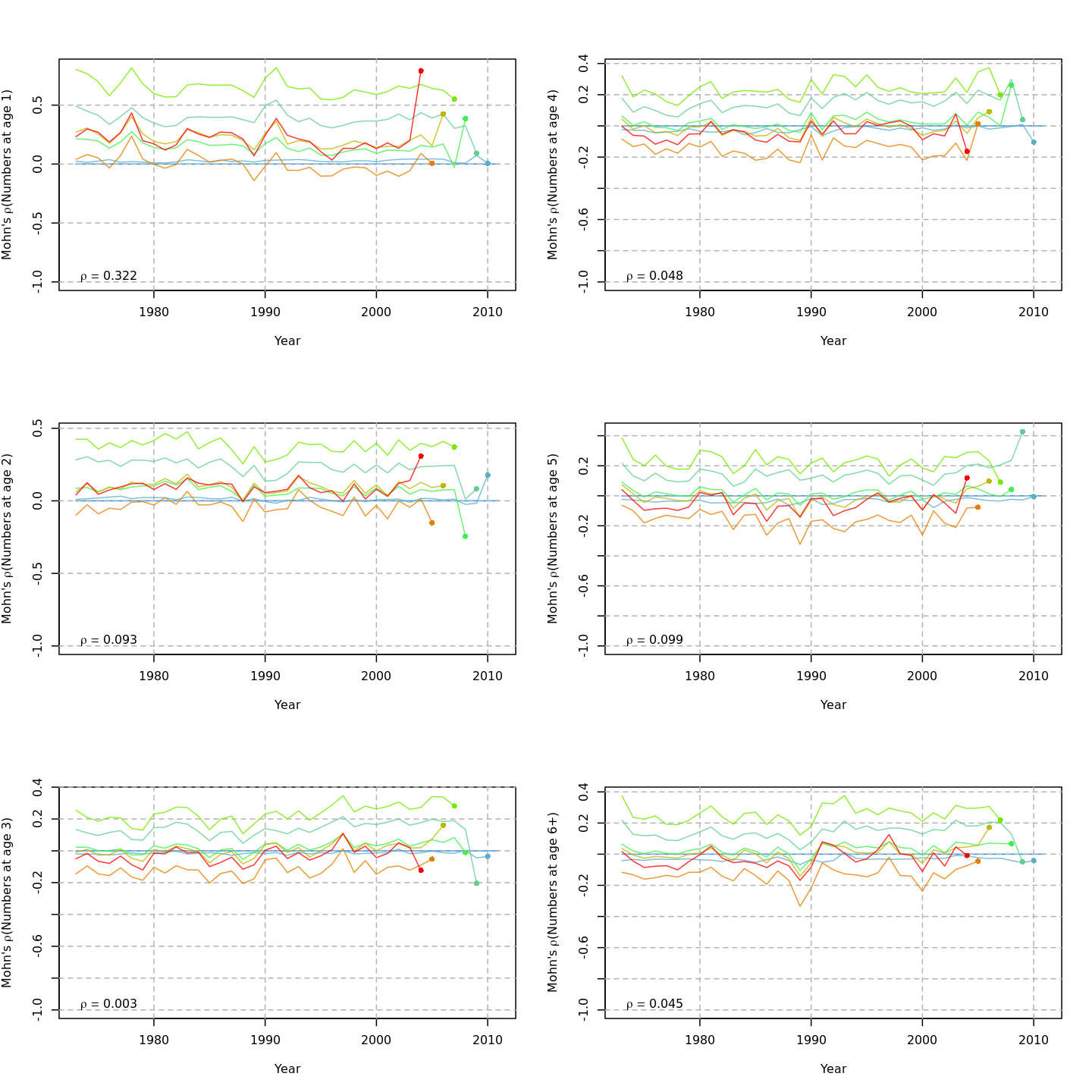 { width=45% }
 { width=45% }
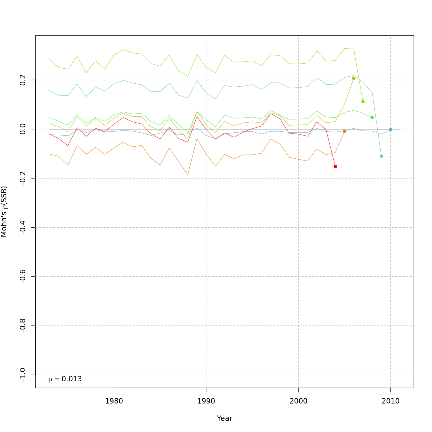 { width=45% }
 { width=45% }
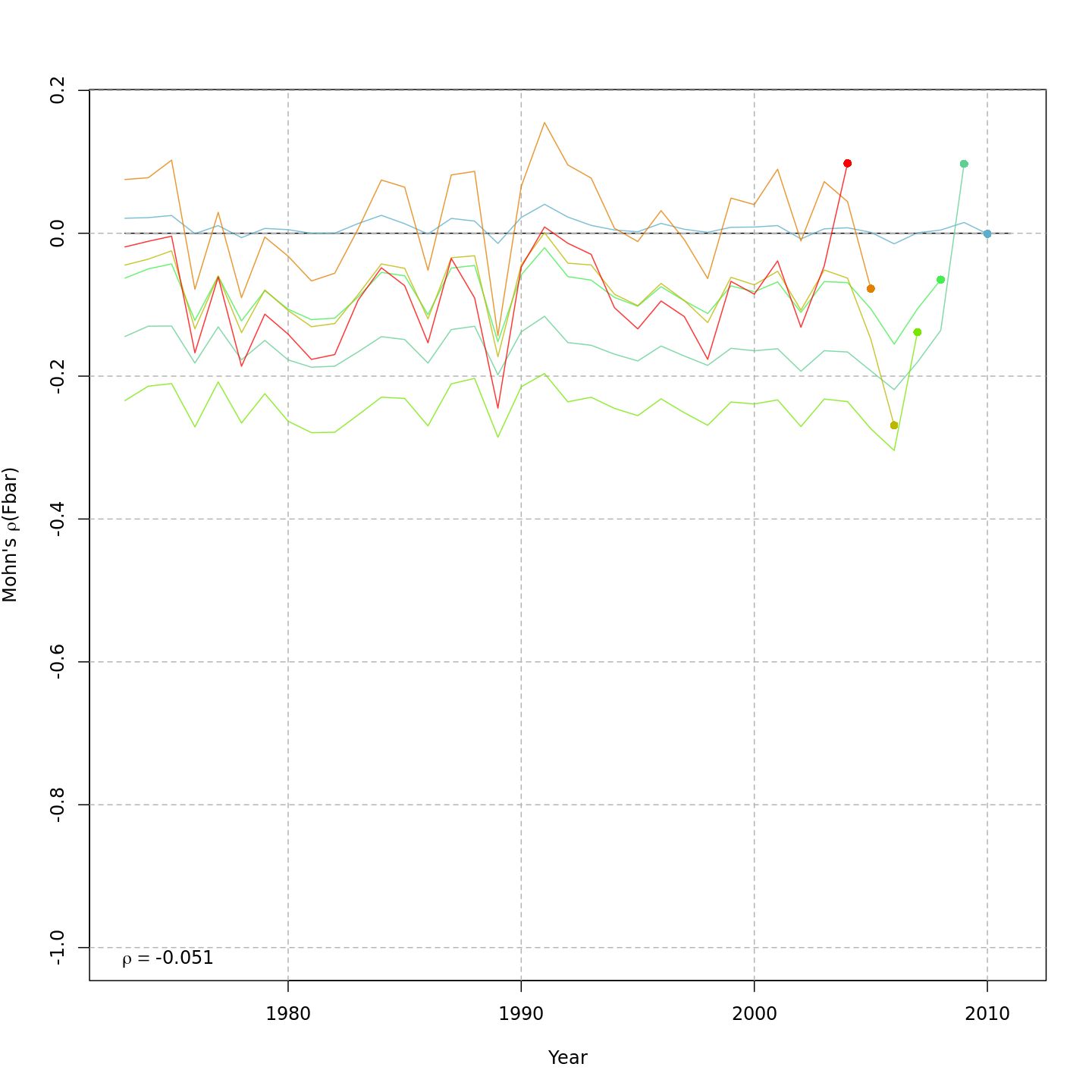 { width=45% }
Model m11 had $\Delta AIC = 1.5$ and the lowest retrospective pattern for all numbers-at-age and F. Model m11 left $M_a$ fixed at the values from the ASAP data file (as in m1) and estimated 2D AR1 deviations around these mean $M_a$. This is how $M$ was modeled in Cadigan (2016).
 { width=45% }
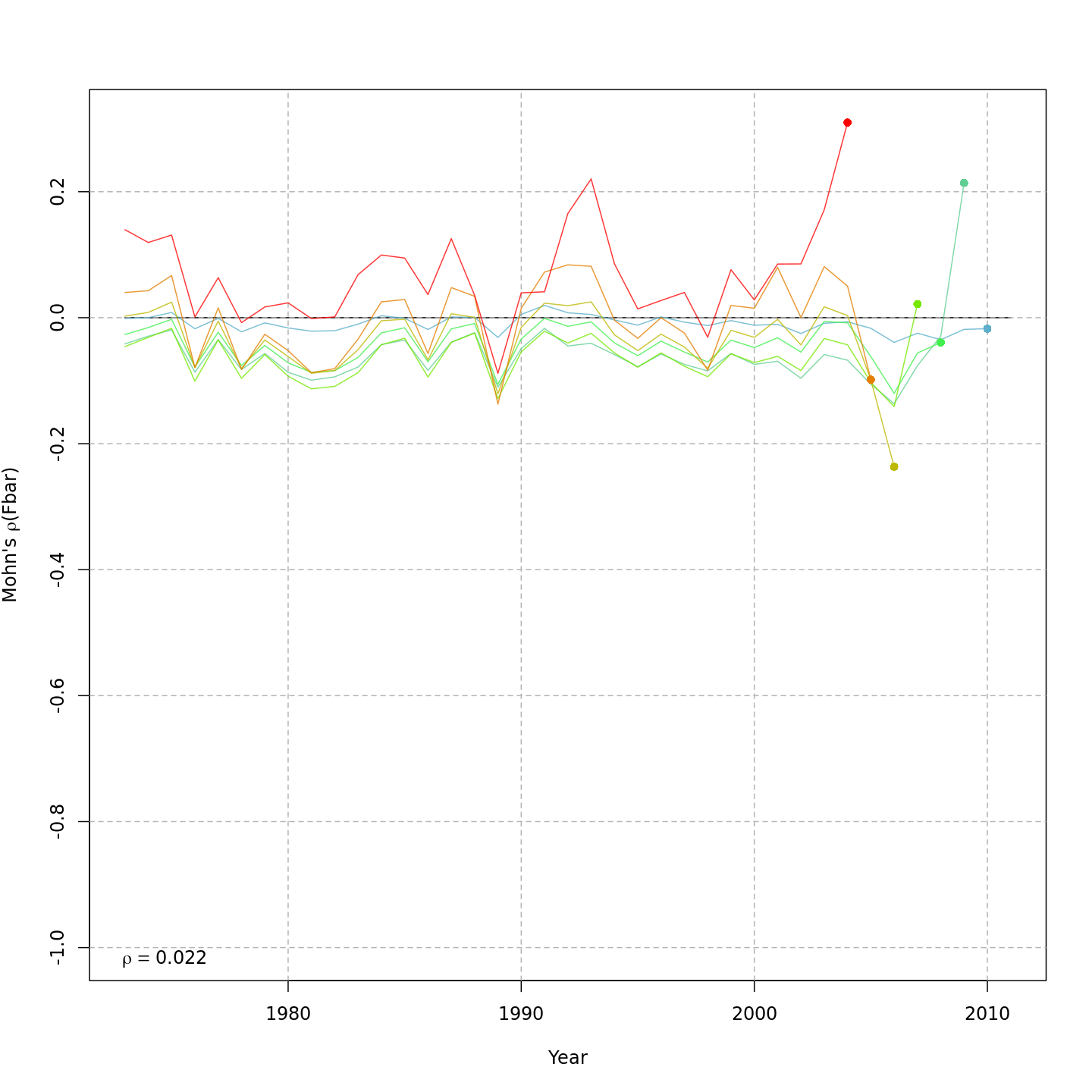 { width=45% }
 { width=45% }
Stock status
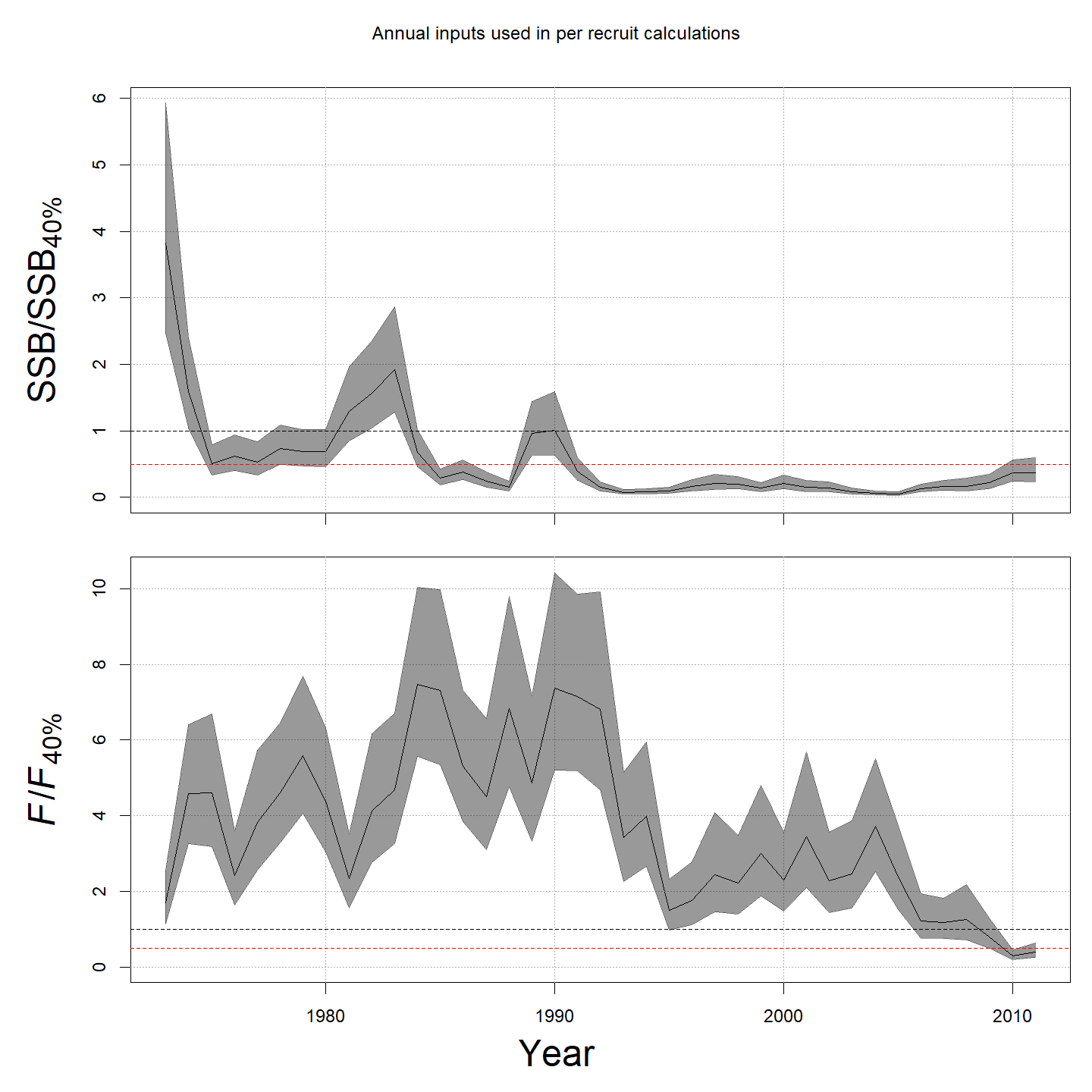
Compared to m1 (left), m8 and m11 (center, right) estimated higher M, lower and more uncertain F, and higher SSB -- a much rosier picture of the stock status through time.
 { width=31% }
 { width=31% }
 { width=31% }
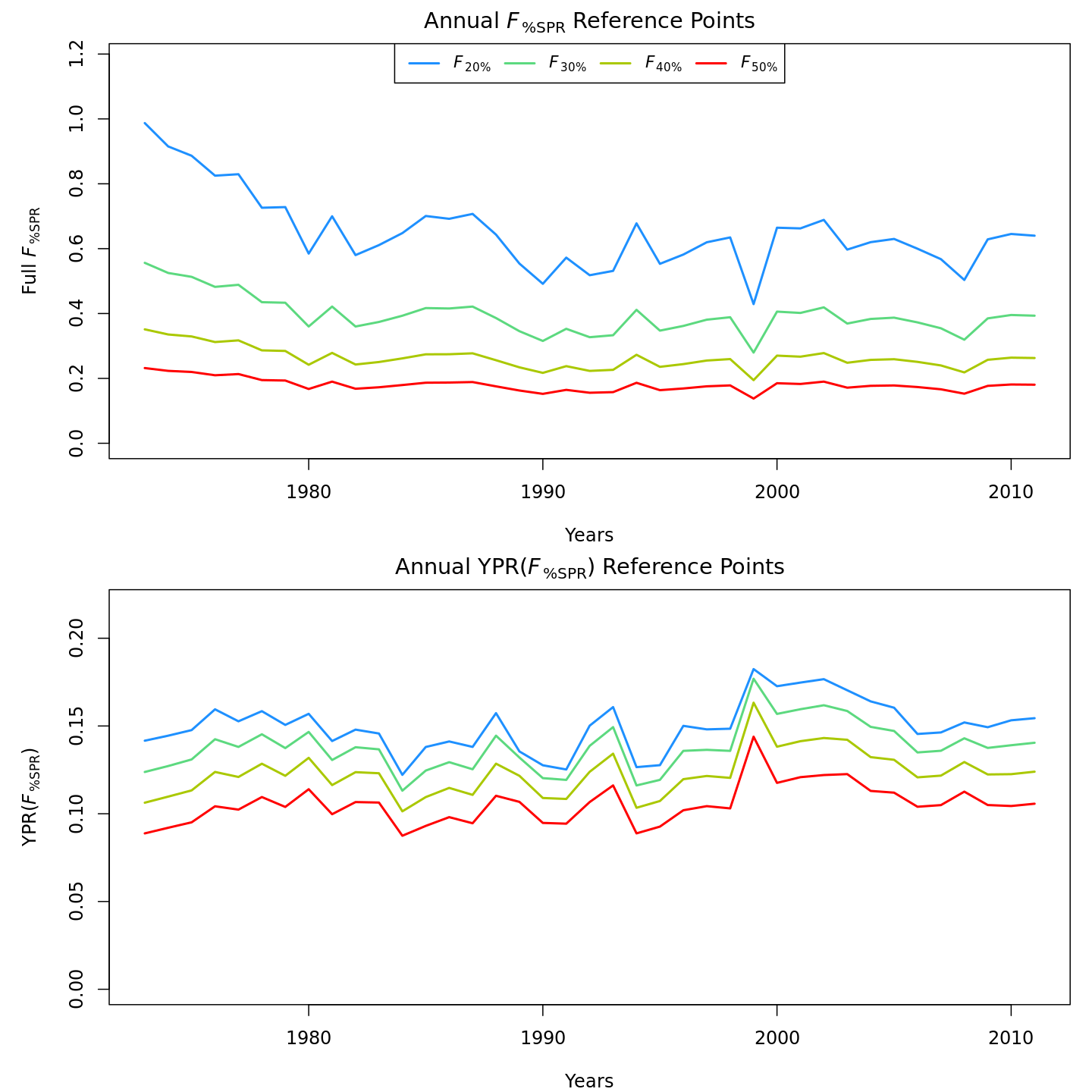
Compared to m1 (left), m8 and m11 (center, right) estimated higher and more variable reference points, $F_{\%SPR}$ (top), and lower and more variable yield-per-recruit (bottom). Model m11 (right) estimated more of a trend in yield-per-recruit and $F_{\%SPR}$, with a notable shift around 1990.
 { width=31% }
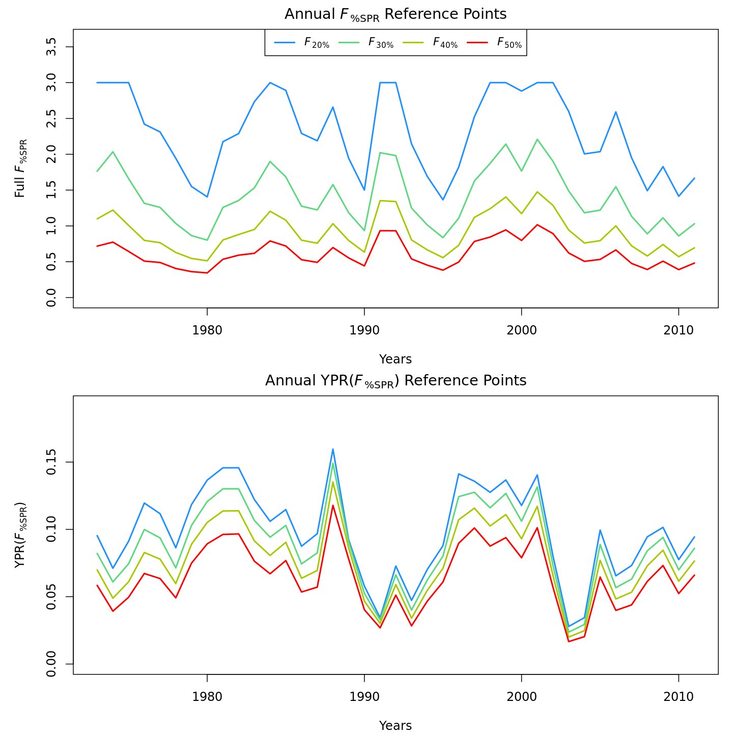 { width=31% }
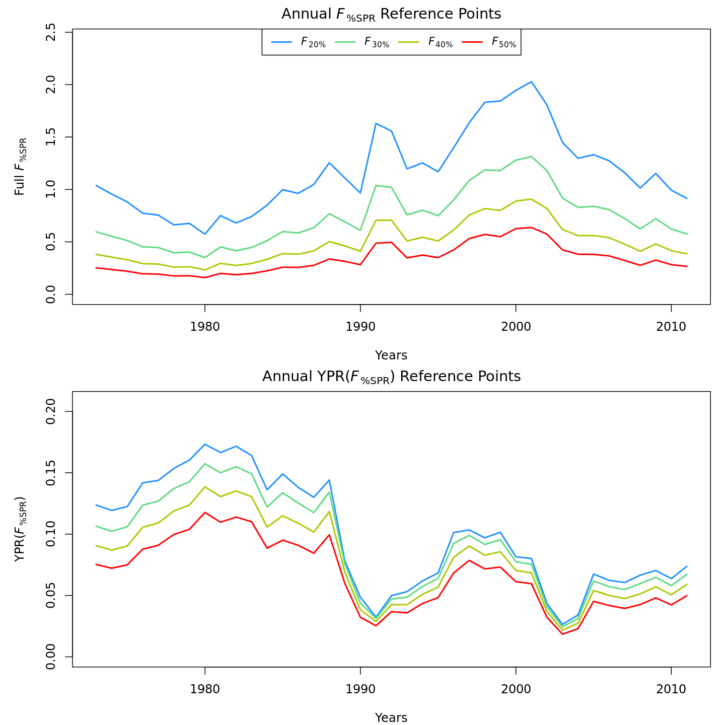 { width=31% }
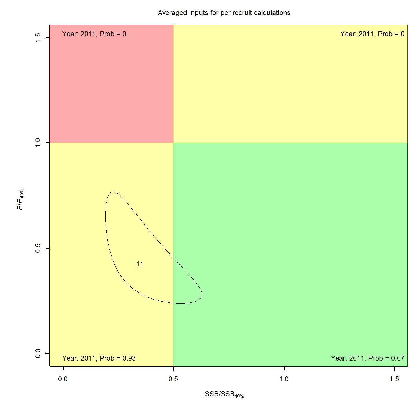
In the final year (2011), m8 and m11 both estimated much lower probabilities of the stock being overfished than m1 (17% and 21% vs. 99%).
 { width=31% }
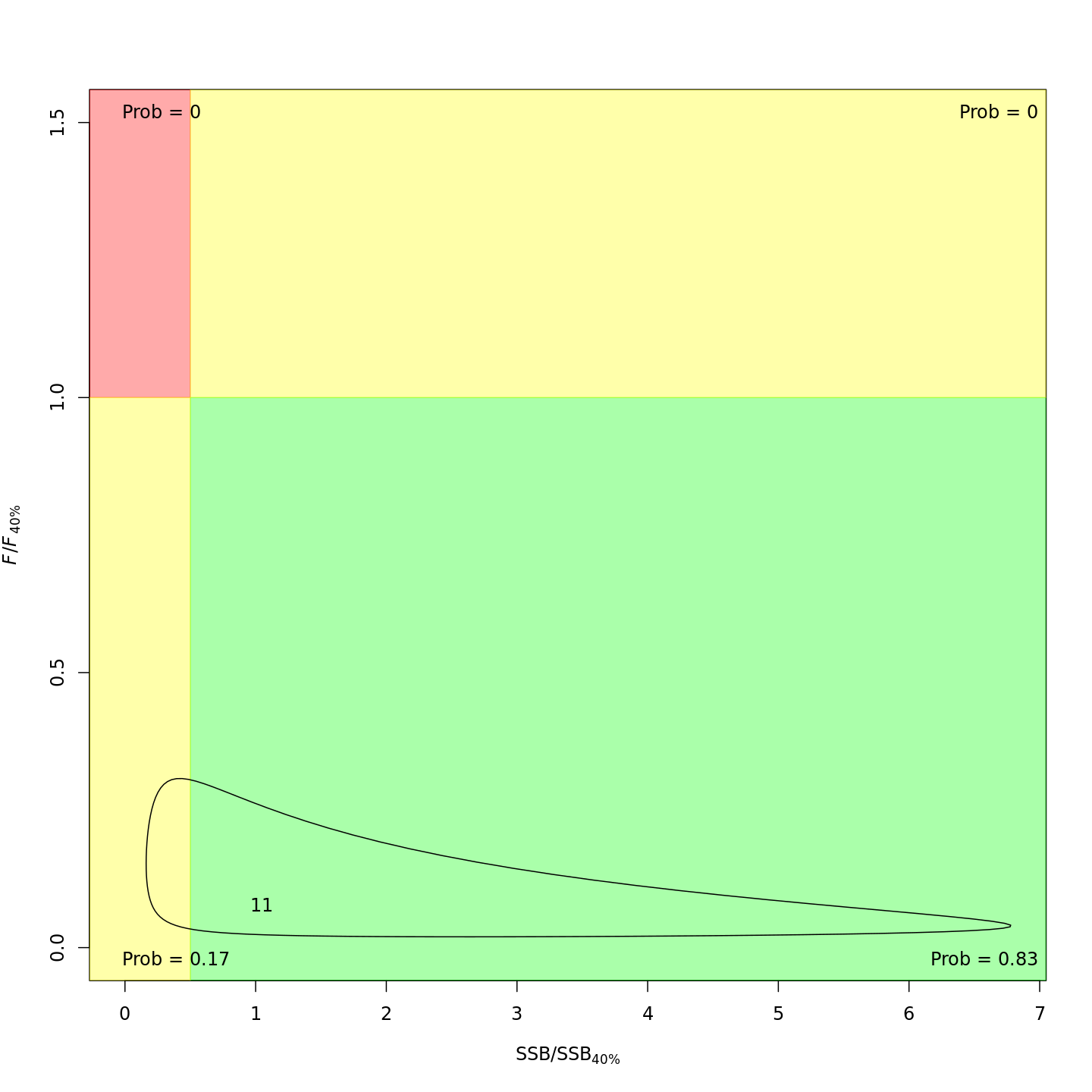 { width=31% }
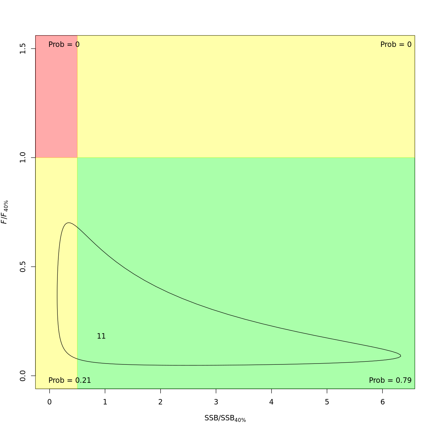 { width=31% }
Yet more M options
If you want to estimate M-at-age shared/mirrored among some but not all ages, you'll need to modify input$map$M_a after calling prepare_wham_input().
timjmiller/wham documentation built on April 28, 2024, 5:39 a.m.
R Package Documentation
Browse R Packages
We want your feedback!
Note that we can't provide technical support on individual packages. You should contact the package authors for that.
knitr::opts_chunk$set( collapse = TRUE, comment = "#>" ) wham.dir <- find.package("wham") knitr::opts_knit$set(root.dir = file.path(wham.dir,"extdata")) library(knitr) library(kableExtra)
In this vignette we walk through an example using the wham (WHAM = Woods Hole Assessment Model) package to run a state-space age-structured stock assessment model. WHAM is a generalization of code written for Miller et al. (2016) and Xu et al. (2018), and in this example we apply WHAM to the same stock, Southern New England / Mid-Atlantic Yellowtail Flounder.
This is the 5th WHAM example, which builds off example 2:
- full state-space model (numbers-at-age are random effects for all ages,
NAA_re = list(sigma='rec+1',cor='iid')) - logistic normal age compositions, pooling zero observations with adjacent ages (
age_comp = "logistic-normal-pool0") - random-about-mean recruitment (
recruit_model = 2) - 5 indices
- fit to 1973-2011 data
We assume you already have wham installed. If not, see the Introduction. The simpler 1st example, without environmental effects or time-varying $M$, is available as a R script and vignette.
In example 5, we demonstrate how to specify and run WHAM with the following options for natural mortality:
- not estimated (fixed at input values)
- one value, $M$
- age-specific, $M_a$ (independent)
- function of weight-at-age, $M_{y,a} = \mu_M * W_{y,a}^b$
- AR1 deviations by age (random effects), $M_{y,a} = \mu_M + \delta_a \quad\mathrm{and}\quad \delta_a \sim \mathcal{N} (\rho_a \delta_{a-1}, \sigma^2_M)$
- AR1 deviations by year (random effects), $M_{y,a} = \mu_M + \delta_y \quad\mathrm{and}\quad \delta_y \sim \mathcal{N} (\rho_y \delta_{y-1}, \sigma^2_M)$
- 2D AR1 deviations by age and year (random effects), $M_{y,a} = M_a + \delta_{y,a} \quad\mathrm{and}\quad \delta_{y,a} \sim \mathcal{N}(0,\Sigma)$
We also demonstrate alternate specifications for the link between $M$ and an environmental covariate, the Gulf Stream Index (GSI), as in O'Leary et al. (2019):
- none
- linear (in log-space), $M_{y,a} = e^{\mathrm{log}\mu_M + \beta_1 E_y}$
- quadratic (in log-space), $M_{y,a} = e^{\mathrm{log}\mu_M + \beta_1 E_y + \beta_2 E^2_y}$
Note that you can specify more than one of the above effects on $M$, although the model may not be estimable. For example, the most complex model with weight-at-age, 2D AR1 age- and year-deviations, and a quadratic environmental effect: $M_{y,a} = e^{\mathrm{log}\mu_M + b W_{y,a} + \beta_1 E_y + \beta_2 E^2_y + \delta_{y,a}}$.
1. Load data
Open R and load the wham package:
library(wham) library(tidyverse) library(viridis)
For a clean, runnable .R script, look at ex5_M_GSI.R in the example_scripts folder of the wham package install:
wham.dir <- find.package("wham") file.path(wham.dir, "example_scripts")
You can run this entire example script with:
write.dir <- "choose/where/to/save/output" # otherwise will be saved in working directory source(file.path(wham.dir, "example_scripts", "ex5_M_GSI.R"))
Let's create a directory for this analysis:
# choose a location to save output, otherwise will be saved in working directory write.dir <- "choose/where/to/save/output" dir.create(write.dir) setwd(write.dir)
We need the same ASAP data file as in example 2, and the environmental covariate (GSI). Let's copy ex2_SNEMAYT.dat and GSI.csv to our analysis directory:
wham.dir <- find.package("wham") file.copy(from=file.path(wham.dir,"extdata","ex2_SNEMAYT.dat"), to=write.dir, overwrite=FALSE) file.copy(from=file.path(wham.dir,"extdata","GSI.csv"), to=write.dir, overwrite=FALSE)
Confirm you are in the correct directory and it has the required data files:
list.files()
Read the ASAP3 .dat file into R and convert to input list for wham:
asap3 <- read_asap3_dat("ex2_SNEMAYT.dat")
Load the environmental covariate (Gulf Stream Index, GSI) data into R:
env.dat <- read.csv("GSI.csv", header=T) head(env.dat)
The GSI does not have a standard error estimate, either for each yearly observation or one overall value. In such a case, WHAM can estimate the observation error for the environmental covariate, either as one overall value, $\sigma_E$, or yearly values as random effects, $\mathrm{log}\sigma_{E_y} \sim \mathcal{N}(\mathrm{log}\sigma_E, \sigma^2_{\sigma_E})$. In this example we choose the simpler option and estimate one observation error parameter, shared across years.
2. Specify models
Now we specify several models with different options for natural mortality:
df.mods <- data.frame(M_model = c(rep("---",3),"age-specific","weight-at-age",rep("constant",5),"---"), M_re = c(rep("none",6),"ar1_y","2dar1","none","none","2dar1"), Ecov_process = rep("ar1",11), Ecov_link = c(0,1,2,rep(0,5),1,2,0), stringsAsFactors=FALSE) n.mods <- dim(df.mods)[1] df.mods$Model <- paste0("m",1:n.mods) df.mods <- df.mods %>% select(Model, everything()) # moves Model to first col
Look at the model table:
df.mods
3. Natural mortality options
Next we specify the options for modeling natural mortality by including an optional list argument, M, to the prepare_wham_input() function (see the prepare_wham_input() help page). M specifies estimation options and can overwrite M-at-age values specified in the ASAP data file. By default (i.e. M is NULL or not included), the M-at-age matrix from the ASAP data file is used (M fixed, not estimated). M is a list with the following entries:
-
$model: Natural mortality model options. -
"constant": estimate a single $M$, shared across all ages and years. "age-specific": estimate $M_a$ independent for each age, shared across years.-
"weight-at-age": estimate $M$ as a function of weight-at-age, $M_{y,a} = \mu_M * W_{y,a}^b$, as in Lorenzen (1996) and Miller & Hyun (2018). -
$re: Time- and age-varying random effects on $M$. -
"none": $M$ constant in time and across ages (default). "iid": $M$ varies by year and age, but uncorrelated."ar1_a": $M$ correlated by age (AR1), constant in time."ar1_y": $M$ correlated by year (AR1), constant by age.-
"2dar1": $M$ correlated by year and age (2D AR1), as in Cadigan (2016). -
$initial_means: Initial/mean M-at-age vector, with length = number of ages (if$model = "age-specific") or 1 (if$model = "weight-at-age"or"constant"). IfNULL, initial mean M-at-age values are taken from the first row of the MAA matrix in the ASAP data file. -
$est_ages: Vector of ages to estimate age-specific $M_a$ (others will be fixed at initial values). E.g. in a model with 6 ages,$est_ages = 5:6will estimate $M_a$ for the 5th and 6th ages, and fix $M$ for ages 1-4. IfNULL, $M$ at all ages is fixed atM$initial_means(if notNULL) or row 1 of the MAA matrix from the ASAP file (ifM$initial_means = NULL). -
$logb_prior: (Only for weight-at-age model) TRUE or FALSE (default), should a $\mathcal{N}(0.305, 0.08)$ prior be used onlog_b? Based on Fig. 1 and Table 1 (marine fish) in Lorenzen (1996).
For example, to fit model m1, fix $M_a$ at values in ASAP file:
M <- NULL # or simply leave out of call to prepare_wham_input
To fit model m6, estimate one $M$, constant by year and age:
M <- list(model="constant", est_ages=1)
And to fit model m8, estimate mean $M$ with 2D AR1 deviations by year and age:
M <- list(model="constant", est_ages=1, re="2dar1")
To fit model m11, use the $M_a$ values specified in the ASAP file, but with 2D AR1 deviations as in Cadigan (2016):
M <- list(re="2dar1")
4. Linking M to an environmental covariate (GSI)
As described in example 2, the environmental covariate options are fed to prepare_wham_input() as a list, ecov. This example differs from example 2 in that:
$logsigma = "est_1": estimate the observation error for the GSI (one overall value for all years). The other option is"est_re"to allow the GSI observation error to have yearly fluctuations (random effects). The Cold Pool Index in example 2 had yearly observation errors given.$lag = 0: GSI in year t affects $M$ in year t, instead of year t+1.$where = "M": GSI affects $M$, instead of recruitment.$how:ecov$how = 0estimates the GSI time-series model (AR1) for models without a GSI-M effect, in order to compare AIC with models that do include a GSI-M effect. Settingecov$how = 1is necessary to allow a GSI-M effect.$link_model: specifies the model linking GSI to $M$. Can beNA(no effect, default),"linear", or"poly-x"(where x is the degree of a polynomial). In this example we demonstrate models with no GSI-M effect, a linear GSI-M effect, and a quadratic GSI-M effect ("poly-2"). WHAM includes a function to calculate orthogonal polynomials in TMB, akin to thepoly()function in R.
For example, the ecov list for model m3 with a quadratic GSI-M effect:
# example for model m3 ecov <- list( label = "GSI", mean = as.matrix(env.dat$GSI), logsigma = 'est_1', # estimate obs sigma, 1 value shared across years year = env.dat$year, use_obs = matrix(1, ncol=1, nrow=dim(env.dat)[1]), # use all obs (=1) lag = 0, # GSI in year t affects M in same year process_model = "ar1", # GSI modeled as AR1 (random walk would be "rw") where = "M", # GSI affects natural mortality how = 1, # include GSI effect on M link_model = "poly-2") # quadratic GSI-M effect
Note that you can set ecov = NULL to fit the model without environmental covariate data, but here we fit the ecov data even for models without GSI effect on $M$ (m1, m4-8) so that we can compare them via AIC (need to have the same data in the likelihood). We accomplish this by setting ecov$how = 0 and ecov$process_model = "ar1".
5. Run all models
All models use the same options for recruitment (random-about-mean, no stock-recruit function) and selectivity (logistic, with parameters fixed for indices 4 and 5).
env.dat <- read.csv("GSI.csv", header=T) for(m in 1:n.mods){ ecov <- list( label = "GSI", mean = as.matrix(env.dat$GSI), logsigma = 'est_1', # estimate obs sigma, 1 value shared across years year = env.dat$year, use_obs = matrix(1, ncol=1, nrow=dim(env.dat)[1]), # use all obs (=1) lag = 0, # GSI in year t affects M in same year process_model = df.mods$Ecov_process[m], # "rw" or "ar1" where = "M", # GSI affects natural mortality how = ifelse(df.mods$Ecov_link[m]==0,0,1), # 0 = no effect (but still fit Ecov to compare AIC), 1 = mean link_model = c(NA,"linear","poly-2")[df.mods$Ecov_link[m]+1]) m_model <- df.mods$M_model[m] if(df.mods$M_model[m] == '---') m_model = "age-specific" if(df.mods$M_model[m] %in% c("constant","weight-at-age")) est_ages = 1 if(df.mods$M_model[m] == "age-specific") est_ages = 1:asap3$dat$n_ages if(df.mods$M_model[m] == '---') est_ages = NULL M <- list( model = m_model, re = df.mods$M_re[m], est_ages = est_ages ) if(m_model %in% c("constant","weight-at-age")) M$initial_means = 0.28 input <- prepare_wham_input(asap3, recruit_model = 2, model_name = paste0("m",m,": ", df.mods$M_model[m]," + ",c("no","linear","poly-2")[df.mods$Ecov_link[m]+1]," GSI link + ",df.mods$M_re[m]," devs"), ecov = ecov, selectivity=list(model=rep("logistic",6), initial_pars=c(rep(list(c(3,3)),4), list(c(1.5,0.1), c(1.5,0.1))), fix_pars=c(rep(list(NULL),4), list(1:2, 1:2))), NAA_re = list(sigma='rec+1',cor='iid'), M=M, age_comp = "logistic-normal-pool0") # logistic normal pool 0 obs # Fit model mod <- fit_wham(input, do.retro=T, do.osa=F) # turn off OSA residuals to save time # Save model saveRDS(mod, file=paste0(df.mods$Model[m],".rds")) # If desired, plot output in new subfolder # plot_wham_output(mod=mod, dir.main=file.path(getwd(),df.mods$Model[m]), out.type='html') # If desired, do projections # mod_proj <- project_wham(mod) # saveRDS(mod_proj, file=paste0(df.mods$Model[m],"_proj.rds")) }
6. Compare models
data(vign5_res) # data(vign5_MAA)
Collect all models into a list.
mod.list <- paste0(df.mods$Model,".rds") mods <- lapply(mod.list, readRDS)
Get model convergence and stats.
opt_conv = 1-sapply(mods, function(x) x$opt$convergence) ok_sdrep = sapply(mods, function(x) if(x$na_sdrep==FALSE & !is.na(x$na_sdrep)) 1 else 0) df.mods$conv <- as.logical(opt_conv) df.mods$pdHess <- as.logical(ok_sdrep)
Only calculate AIC and Mohn's rho for converged models.
df.mods$runtime <- sapply(mods, function(x) x$runtime) df.mods$NLL <- sapply(mods, function(x) round(x$opt$objective,3)) not_conv <- !df.mods$conv | !df.mods$pdHess mods2 <- mods mods2[not_conv] <- NULL df.aic.tmp <- as.data.frame(compare_wham_models(mods2, sort=FALSE, calc.rho=T)$tab) df.aic <- df.aic.tmp[FALSE,] ct = 1 for(i in 1:n.mods){ if(not_conv[i]){ df.aic[i,] <- rep(NA,5) } else { df.aic[i,] <- df.aic.tmp[ct,] ct <- ct + 1 } } df.aic[,1:2] <- format(round(df.aic[,1:2], 1), nsmall=1) df.aic[,3:5] <- format(round(df.aic[,3:5], 3), nsmall=3) df.aic[grep("NA",df.aic$dAIC),] <- "---" df.mods <- cbind(df.mods, df.aic)
Make results table prettier.
df.mods$Ecov_link <- c("---","linear","poly-2")[df.mods$Ecov_link+1] df.mods$M_re[df.mods$M_re=="none"] = "---" colnames(df.mods)[2] = "M_est" rownames(df.mods) <- NULL
Look at results table.
df.mods
7. Results
In the table, I have highlighted models which converged and successfully inverted the Hessian to produce SE estimates for all (fixed effect) parameters. WHAM stores this information in mod$na_sdrep (should be FALSE), mod$sdrep$pdHess (should be TRUE), and mod$opt$convergence (should be 0). See stats::nlminb() and TMB::sdreport() for details.
Models m8 (estimate mean $M$ and 2D AR1 deviations by year and age, no GSI effect) and m11 (keep mean $M$ fixed but estimate 2D AR1 deviations) had the lowest AIC and were overwhelmingly supported relative to the other models (bold in table below).
library(knitr) library(kableExtra) # vign5_res[,12:14] = round(vign5_res[,12:14], 3) posdef = which(vign5_res$pdHess == TRUE) thebest = c(8,11) vign5_res %>% # mutate(na_sdrep = cell_spec(na_sdrep, "html", bold = ifelse(na_sdrep == TRUE,TRUE,FALSE))) %>% # select(everything()) %>% dplyr::rename("M model"="M_est", "GSI"="Ecov_process", "GSI link"="Ecov_link", "Converged"="conv", "Pos def\nHessian"="pdHess", "Runtime\n(min)"="runtime", "$\\rho_{R}$"="rho_R", "$\\rho_{SSB}$"="rho_SSB", "$\\rho_{\\overline{F}}$"="rho_Fbar") %>% kable(escape = F) %>% kable_styling(bootstrap_options = c("condensed","responsive")) %>% row_spec(posdef, background = gray.colors(10,end=0.95)[10]) %>% row_spec(thebest, bold=TRUE)
Estimated M
- Models allowed to estimate mean $M$ increased $M$ compared to the fixed values in
m1-3(more green/yellow than blue). - Models that estimated $M_a$ had highest $M_a$ for ages 4-5.
- Models that estimated $M_y$ had higher $M_y$ in the early 1990s and around 2000.
Below is a plot of $M$ by age (y-axis) and year (x-axis) for all models. Models with a positive definite Hessian are solid, and models with non-positive definite Hessian are pale.
{ width=90% }
Retrospective patterns
Compared to m1, the retrospective pattern for m8 was slightly worse for recruitment (m8 0.32, m1 0.23) but improved for SSB (m8 0.01, m1 0.07) and F (m8 -0.05, m1 -0.11). In general, models with GSI effects or 2D AR1 deviations on $M$ had reduced retrospective patterns compared to the status quo (m1) and models with 1D AR1 random effects on $M$. Compare the retrospective patterns of numbers-at-age, SSB, and F for models m1 (left, fixed $M_a$) and m8 (right, estimated $M$ + 2D AR1 deviations).
{ width=45% }{ width=45% }
{ width=45% }{ width=45% }
{ width=45% }{ width=45% }
Model m11 had $\Delta AIC = 1.5$ and the lowest retrospective pattern for all numbers-at-age and F. Model m11 left $M_a$ fixed at the values from the ASAP data file (as in m1) and estimated 2D AR1 deviations around these mean $M_a$. This is how $M$ was modeled in Cadigan (2016).
{ width=45% }{ width=45% }
{ width=45% }
Stock status
Compared to m1 (left), m8 and m11 (center, right) estimated higher M, lower and more uncertain F, and higher SSB -- a much rosier picture of the stock status through time.
{ width=31% }{ width=31% }{ width=31% }
Compared to m1 (left), m8 and m11 (center, right) estimated higher and more variable reference points, $F_{\%SPR}$ (top), and lower and more variable yield-per-recruit (bottom). Model m11 (right) estimated more of a trend in yield-per-recruit and $F_{\%SPR}$, with a notable shift around 1990.
{ width=31% }{ width=31% }{ width=31% }
In the final year (2011), m8 and m11 both estimated much lower probabilities of the stock being overfished than m1 (17% and 21% vs. 99%).
{ width=31% }{ width=31% }{ width=31% }
Yet more M options
If you want to estimate M-at-age shared/mirrored among some but not all ages, you'll need to modify input$map$M_a after calling prepare_wham_input().
R Package Documentation
Browse R Packages
We want your feedback!
Note that we can't provide technical support on individual packages. You should contact the package authors for that.
Embedding an R snippet on your website
Add the following code to your website.
For more information on customizing the embed code, read Embedding Snippets.