Latent Environmental & Genetic InTeraction (LEGIT) modelling"
In LEGIT: Latent Environmental & Genetic InTeraction (LEGIT) Model

Note that you can cite this work as:

Jolicoeur-Martineau, A., Wazana, A., Szekely, E., Steiner, M., Fleming, A. S., Kennedy, J. L., Meaney M. J. & Greenwood, C.M. (2017). Alternating optimization for GxE modelling with weighted genetic and environmental scores: examples from the MAVAN study. arXiv preprint arXiv:1703.08111.

The LEGIT model

The Latent Environmental & Genetic InTeraction (LEGIT) model is an interaction model with two latent variables: $\mathbf{g}$ a weighted sum of genetic variants (genetic score) and $\mathbf{e}$ a weighted sum of environmental variables (environmental score).

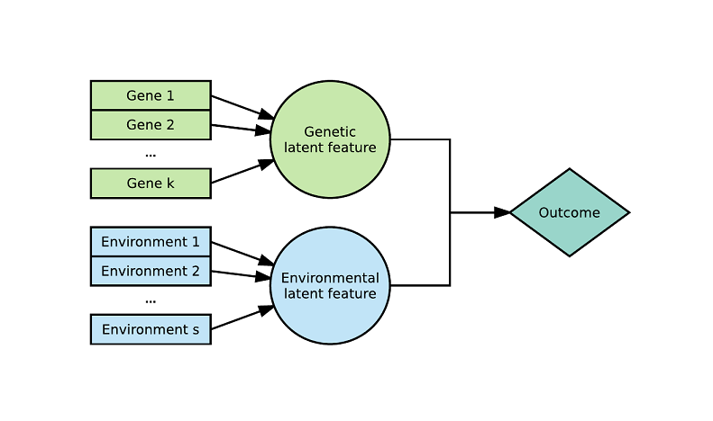
Assuming $\mathbf{g}_1$,...,$\mathbf{g}_k$ are $k$ genetic variants of interest, generally represented as the number of dominant alleles (0, 1, 2) or the absence or presence of a dominant allele (0, 1) and $\mathbf{e}_1$,...,$\mathbf{e}_s$ are $s$ environments of interest, generally represented as ordinal scores (0, 1, 2 ...) or continuous variables. We define the genetic score $\mathbf{g}$ and environmental score $\mathbf{e}$ as:

$$\mathbf{g}=\sum_{i=1}^{k} p_i \mathbf{g}j $$ $$\mathbf{e}=\sum{l=1}^{s} q_l \mathbf{e}l $$ where $\|p\|_1=\sum{i=1}^{k}p_j=1$ and $\|q\|1= \sum{l=1}^{s}q_l=1$. The weights can be interpreted as the relative contributions of each genetic variant or environment.

The weights of these scores are estimated within a generalized linear model of the form :

$$\mathbf{E}[\mathbf{y}] = g^{-1}(f(\mathbf{g},\mathbf{e},X|\beta)+X_{covs} \beta_{covs})$$ where $g$ is the link function, $f$ is a linear function between $\mathbf{g}$, $\mathbf{e}$ and other variables from the matrix $X$ and $X_{covs}$ is a matrix of additionnal covariates.

Although this approach was originally made for GxE modelling, it is flexible and does not require the use of genetic and environmental variables. It can also handle more than 2 latent variables (rather than just G and E) and 3-way interactions or more.

For a two-way $G\times E$ model, we would define $f$ as:

$$f(\mathbf{g},\mathbf{e},X|\beta) = \beta_0+\beta_e \mathbf{e}+\beta_g \mathbf{g}+\beta_{eg} \mathbf{e}\mathbf{g}$$

For a three-way $G\times E \times Z$ model, we would define $f$ as:

$$f(\mathbf{g},\mathbf{e},X|\beta) = \beta_0+\beta_e \mathbf{e}+\beta_g \mathbf{g}+\beta_z \mathbf{z}+\beta_{eg} \mathbf{eg}+\beta_{ez} \mathbf{ez}+\beta_{zg} \mathbf{zg}+\beta_{egz} \mathbf{egz}$$

Examples of LEGIT models

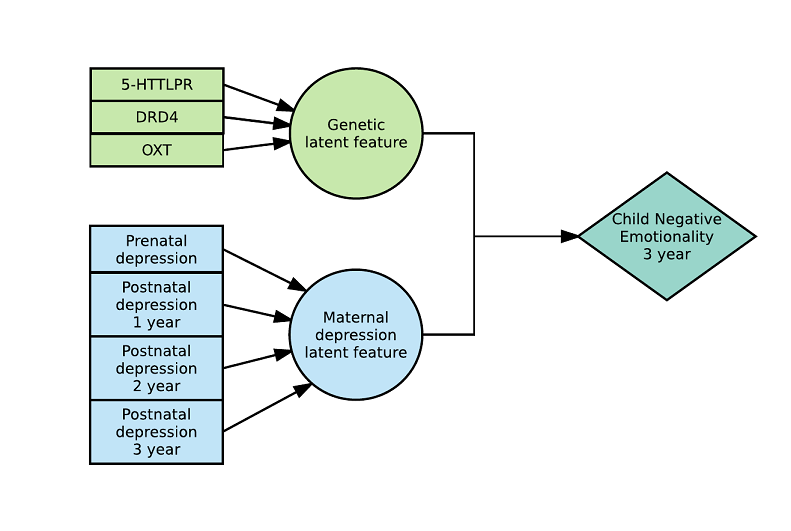
Here is an example with 2 latent variables and a 2-way interaction (see arxiv) :

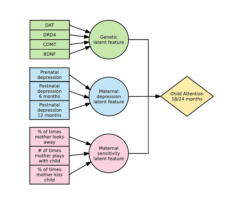
Here is an example with 3 latent variables and a 3-way interaction (see arxiv) :

Algorithm

Full details of the algorithm are available on arXiv.

Implementation

In the LEGIT package, we include the following functions:

To fit a LEGIT model with 2 latent variables (G and E)

LEGIT: Fits a LEGIT model
plot.LEGIT: Plot function for LEGIT models.
predict.LEGIT: Predictions of LEGIT fits.
summary.LEGIT: Summarizing LEGIT fits.
LEGIT_cv: Uses cross-validation on a LEGIT model.
stepwise_search: Adds the best variable or drops the worst variable one at a time in the genetic or environmental score of a LEGIT model.
GxE_interaction_test: Testing of the GxE interaction, a method adapted from Belsky, Pluess et Widaman (2013). Reports the different hypotheses (diathesis-stress/vantage-sensitivity vs differential susceptibility), assuming or not assuming a main effect for E (WEAK vs STRONG) using the LEGIT model.

To fit a IMLEGIT model (LEGIT model with more than 2 latent variables)

IMLEGIT: Fits a IMLEGIT model.
predict.IMLEGIT: Predictions of IMLEGIT fits.
summary.IMLEGIT: Summarizing IMLEGIT fits.
IMLEGIT_cv: Uses cross-validation on a IMLEGIT model.
stepwise_search_IM: Adds the best variable or drops the worst variable one at a time in the genetic or environmental score of a IMLEGIT model.
bootstrap_var_select: Creates bootstrap samples, run stepwise search on all of them and then report the percentage of times that each variables were selected.
genetic_var_select: Parallel genetic algorithm variable selection.

To simulate examples of GxE models

example_2way: Simulated example of a 2 way interaction GxE model (where G and E are latent variables).
example_3way: Simulated example of a 3 way interaction GxExz model (where G and E are latent variables).
example_3way_3latent: Simulated example of a 3 way interaction GxExZ model (where G, E and Z are latent variables).
example_with_crossover: Simulated example of a 2 way interaction GxE model with cross-over point (where G and E are latent variables).

Others

longitudinal_folds: Function to create folds adequately for longitudinal datasets by forcing every observation with the same id to be in the same fold. Can be used with LEGIT_cv to make sure that the cross-validation folds are appropriate when using longitudinal data.

Notes

Interactions inside the genetic and environmental scores must be manually coded as new variables (ex: g1, g2, g1_g2 where g1_g2=g1*g2).
Default starting point is set to $1/k$ for each of the genetic variants and $1/s$ for each of the environmental variables.
Only local convergence is guaranteed, therefore it is recommended to try different starting points.

How to use the LEGIT package: Example 1

Let's look at a three-way interaction model with continuous outcome:

$$\mathbf{g}_j \sim Binomial(n=1,p=.30) \ j = 1, 2, 3, 4$$ $$\mathbf{e}_l \sim Normal(\mu=0,\sigma=1.5) \ l = 1, 2, 3$$ $$\mathbf{z} \sim Normal(\mu=3,\sigma=1)$$ $$\mathbf{g} = .2\mathbf{g}_1 + .15\mathbf{g}_2 - .3\mathbf{g}_3 + .1\mathbf{g}_4 + .05\mathbf{g}_1\mathbf{g}_3 + .2\mathbf{g}_2\mathbf{g}_3 $$ $$ \mathbf{e} = -.45\mathbf{e}_1 + .35\mathbf{e}_2 + .2\mathbf{e}_3$$ $$\mathbf{\mu} = -2 + 2\mathbf{g} + 3\mathbf{e} + \mathbf{z} + 5\mathbf{ge} + 2\mathbf{gz} - 1.5\mathbf{ez} + 2\mathbf{gez} $$ $$ y \sim Normal(\mu,\sigma=1)$$

Let's load the package and look at the dataset.

library(LEGIT)
example_3way(N=5, sigma=1, logit=FALSE, seed=7)

Currently "data" contains the outcome, the true outcome without the noise and the covariate $z$. This dataset should always contain the outcome and all covariates (except for the genes and environments from $\mathbf{g}$ and $\mathbf{e}$)."G" contains the genetic variants and "E" contains the environments. This is all you need to fit a LEGIT model.

We generate N=250 training observations and 100 test observations.

train = example_3way(N=250, sigma=1, logit=FALSE, seed=7)
test = example_3way(N=100, sigma=1, logit=FALSE, seed=6)

We fit the model with the default starting point.

fit_default = LEGIT(train$data, train$G, train$E, y ~ G*E*z)
summary(fit_default)

This is very close to the original model. We can now use the test dataset to find the validation $R^2$.

ssres = sum((test$data$y - predict(fit_default, test$data, test$G, test$E))^2)
sstotal = sum((test$data$y - mean(test$data$y))^2)
R2 = 1 - ssres/sstotal
R2

We can also plot the model at specific values of z.

cov_values = c(3)
names(cov_values) = "z"
plot(fit_default, cov_values = cov_values,cex.leg=1.4, cex.axis=1.5, cex.lab=1.5)

Now, let's see what happens if we introduce variables that are not in the model. Let's add these irrelevant genetic variants:

$$\mathbf{g'}_b \sim Binomial(n=1,p=.30) \ b = 1, 2, 3, 4, 5$$

g1_bad = rbinom(250,1,.30)
g2_bad = rbinom(250,1,.30)
g3_bad = rbinom(250,1,.30)
g4_bad = rbinom(250,1,.30)
g5_bad = rbinom(250,1,.30)
train$G = cbind(train$G, g1_bad, g2_bad, g3_bad, g4_bad, g5_bad)

Let's do a forward search of the genetic variants using the BIC and see if we can recover the right subset of variables.

forward_genes_BIC = stepwise_search(train$data, genes_extra=train$G, env_original=train$E, formula=y ~ E*G*z, search_type="forward", search="genes", search_criterion="BIC", interactive_mode=FALSE)

We recovered the right subset! Now what if we did a backward search using the AIC?

backward_genes_AIC = stepwise_search(train$data, genes_original=train$G, env_original=train$E, formula=y ~ E*G*z, search_type="backward", search="genes", search_criterion="AIC", interactive_mode=FALSE)

We deleted the irrevelant genes and obtained the right subset of variables! The stepwise_search function also has an interactive mode where the user decides which variable should be added/dropped at every step. We can only show the first iteration because the algorithm does'nt receive an input from the user in the vignette but normally you can control the variables added or removed from the stepwise search. This is what the interactive mode looks like:

forward_genes_BIC = stepwise_search(train$data, genes_extra=train$G, env_original=train$E, formula=y ~ E*G*z, search_type="bidirectional-forward", search="genes", search_criterion="BIC", interactive_mode=TRUE)

Manually forcing $\mathbf{g}_3$ inclusion since the interactive mode cannot progress without a user, we get that the second iteration is:

forward_genes_BIC = stepwise_search(train$data, genes_original=train$G[,3,drop=FALSE], genes_extra=train$G[,-3], env_original=train$E, formula=y ~ E*G*z, search_type="bidirectional-forward", search="genes", search_criterion="BIC", interactive_mode=TRUE)

With the interactive mode, you can try alternative pathways, rather than simply adding/dropping the best/worst variable everytime.

How to use the LEGIT package: Example 2

Let's take a quick look at a simple two-way example with binary outcome:

$$\mathbf{g}_j \sim Binomial(n=1,p=.30) \ j = 1, 2, 3, 4$$ $$\mathbf{e}_l \sim Normal(\mu=0,\sigma=1.5) \ l = 1, 2, 3$$ $$\mathbf{g} = .2\mathbf{g}_1 + .15\mathbf{g}_2 - .3\mathbf{g}_3 + .1\mathbf{g}_4 + .05\mathbf{g}_1\mathbf{g}_3 + .2\mathbf{g}_2\mathbf{g}_3 $$ $$ \mathbf{e} = -.45\mathbf{e}_1 + .35\mathbf{e}_2 + .2\mathbf{e}_3$$ $$\mathbf{\mu} = -1 + 2\mathbf{g} + 3\mathbf{e} + 4\mathbf{ge} $$ $$ y \sim Binomial(n=1,p=logit(\mu))$$

We generate N=1000 training observations.

library(LEGIT)
train = example_2way(N=1000, logit=TRUE, seed=777)

We fit the model with the default starting point.

fit_default = LEGIT(train$data, train$G, train$E, y ~ G*E, family=binomial)
summary(fit_default)

We are a little off, especially with regards to the weights of the genetic variants. This is because there is substantial loss of information with binary outcomes. To assess the quality of the fit, we are going to do a 5-Folds cross-validation.

cv_5folds_bin = LEGIT_cv(train$data, train$G, train$E, y ~ G*E, cv_iter=1, cv_folds=5, classification=TRUE, family=binomial, seed=777)
pROC::plot.roc(cv_5folds_bin$roc_curve[[1]])

Although the weights of the genetic variants are a bit off, the model predictive power is good.

We can also plot the model.

plot(fit_default, cex.leg=1.4, cex.axis=1.5, cex.lab=1.5)

How to use the LEGIT package: Example 3

In example 1 we looked at a 3-way model but only two of the three variables were latent. Let's construct the model another time but this time with three latent variables:

$$\mathbf{g}_j \sim Binomial(n=1,p=.30) \ j = 1, 2, 3, 4$$ $$\mathbf{e}_l \sim Normal(\mu=0,\sigma=1.5) \ l = 1, 2, 3$$ $$\mathbf{z}_t \sim Normal(\mu=3,\sigma=1)$$ $$\mathbf{g} = .2\mathbf{g}_1 + .15\mathbf{g}_2 - .3\mathbf{g}_3 + .1\mathbf{g}_4 + .05\mathbf{g}_1\mathbf{g}_3 + .2\mathbf{g}_2\mathbf{g}_3 $$ $$ \mathbf{e} = -.45\mathbf{e}_1 + .35\mathbf{e}_2 + .2\mathbf{e}_3$$ $$ \mathbf{z} = .15\mathbf{z}_1 + .60\mathbf{z}_2 + .25\mathbf{z}_3$$ $$\mathbf{\mu} = -2 + 2\mathbf{g} + 3\mathbf{e} + \mathbf{z} + 5\mathbf{ge} + 2\mathbf{gz} - 1.5\mathbf{ez} + 2\mathbf{gez} $$ $$ y \sim Normal(\mu,\sigma=1)$$

Let's load the package and look at the dataset.

library(LEGIT)
example_3way_3latent(N=5, sigma=1, logit=FALSE, seed=7)

Currently "data" contains the outcome and the true outcome without the noise. This dataset should always contain the outcome and all covariates not included in latent_var.The latent variables are called "G", "E" and "Z" respectively.

We generate N=250 training observations.

train = example_3way_3latent(N=250, sigma=1, logit=FALSE, seed=7)

We fit the model with the default starting point.

fit_default = IMLEGIT(train$data, train$latent_var, y ~ G*E*Z)
summary(fit_default)

Let's add irrelevant genes and try a forward search as before. Note that search = 1 means that we will search for the first latent variable which is "G". We could also set search = 0 to search through all latent variables.

$$\mathbf{g'}_b \sim Binomial(n=1,p=.30) \ b = 1, 2, 3, 4, 5$$

g1_bad = rbinom(250,1,.30)
g2_bad = rbinom(250,1,.30)
g3_bad = rbinom(250,1,.30)
g4_bad = rbinom(250,1,.30)
g5_bad = rbinom(250,1,.30)
G_new = cbind(g1_bad, g2_bad, g3_bad, g4_bad, g5_bad)
forward_genes_BIC = stepwise_search_IM(train$data, latent_var_original=train$latent_var, latent_var_extra=list(G=G_new, E=NULL, Z=NULL), formula=y ~ E*G*Z, search_type="forward", search=1, search_criterion="BIC", interactive_mode=FALSE)