README.md
In Beuleup93/dgrGlm: Regression logistic binary tools
dgrGlm: GRadient Descent For Logistic Regression
DESCRIPTION
This project is part of our training in Data Science at the University of Lyon 2. The main objective is to develop an R package under S3 that allows to do binary
logistic regression distributed on the different cores of the user's computer. Gradient descent is used for the optimization of the parameters.
Here the idea is to allow the user to take advantage of the totality of these computer resources, if of course this can help to make the execution
of the calculations faster. Here are the different functionalities of our package that we will present in the following lines:
- Binary logistic regression model in sequential mode
- Splitting of calculations and data for parallel execution
- Binary logistic regression model in parallel mode
- Comparison of model predictions
- Automatic Features selection
- Model Microbenchmark
- Elasticnet (Ridge and Lasso)
- Multinomiale logistic regression
- Recoding of the target variable (One vs All)
Logistic Regression
Logistic regression is an old and well-known statistical predictive method that applies to binary classification, but can be easily extended to the multiclass
framework (multinomial regression in particular, but not only...).It has become popular in recent years in machine learning thanks to "new" computational
algorithms (optimization) and powerful libraries.
The work on regularization makes its use efficient in the context of high dimensional learning (nb. Var. Expl. >> nb. Obsv.). It is related to neural networks
(simple perceptron).
The objective of this guide is not to explain the mathematical formulas around logistic regression but to give you an overview of our package.
Installation and data loading
In order to use our package, you should install it from Github.
library(devtools)
install_github("Beuleup93/dgrGlm")
Once the package is downloaded and successfully installed, please load it for use.
library(dgrGlm)
Now you can access all available functions of the package. To prove it, we will display the documentation of our fit function.
you can write in your console: ?dgrGlm.fit to see the documentation or:
help(dgrGlm.fit)
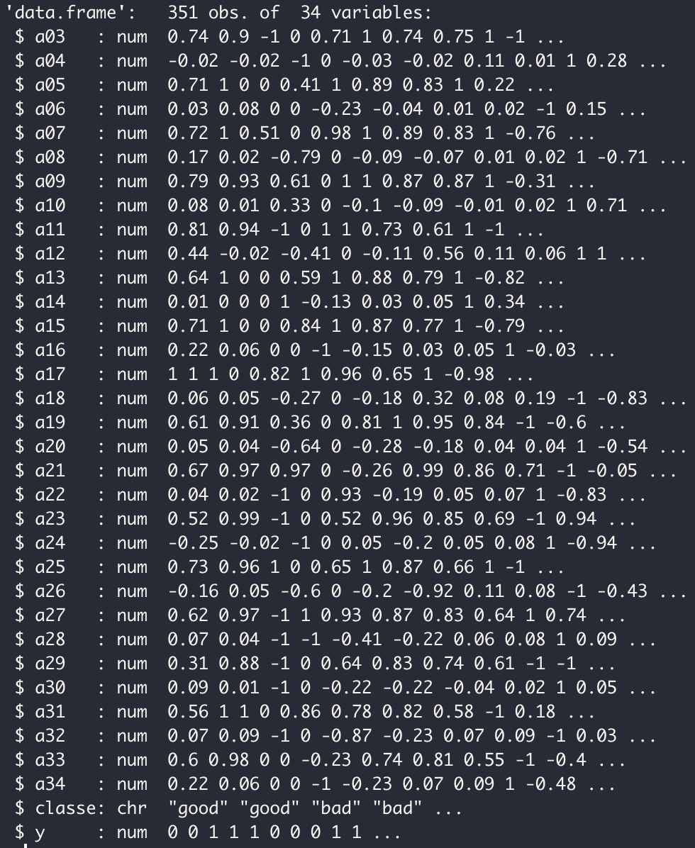
In order to test our functions, we will work with the dataset ionosphere.xlsx. It consists of 351 obervations and 34 variables.
1. Binary Logistic Regression
We will start by testing the binary logistic regression on our dataset. The variable to be explained is Y and the explicatives variables are a03,...,a34.
General function fit
dgrglm.fit <- function(formule, data, ncores=NA, mode_compute="parallel", leaning_rate=0.1,
                       max_iter=100, tolerance=1e-04, batch_size=NA,
                       random_state=102, centering = FALSE, feature_selection=FALSE,
                       p_value=0.01, rho=0.1, C=0.1, iselasticnet=FALSE){...}
This function takes into account several aspects:
- sequential execution with mode_compute="sequentiel"
- parallel execution with for example ncores=4, and mode_compute="parallel"
- Execution in Batch, Mini Batch and Online modes with batch_size=NA
- Centering reduction of explanatory variables with centering = TRUE
- Selection of variables by playing on the arguments feature_selection=TRUE, p_value=0.01
- Elasticnet (Ridge for rho=0 and Lasso for rho=1) avec les arguments C et rho.
For each algorithm the principle is explained in the report.
sequential execution:
For a sequential execution, specify comput_mode ='sequentiel'.
- BATCH Mode
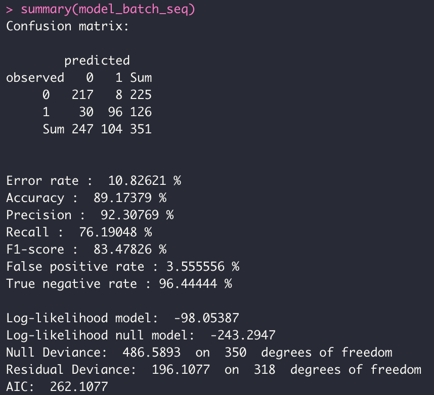
model_batch_seq <- dgrglm.fit(y~., data = data, mode_compute="sequentiel",
leaning_rate=0.1, max_iter=1000,tolerance=1e-06)
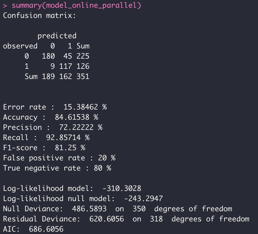
summary(model_batch_seq)
We have overloaded the print and summary methods for a display adapted to our objects returned by fit.
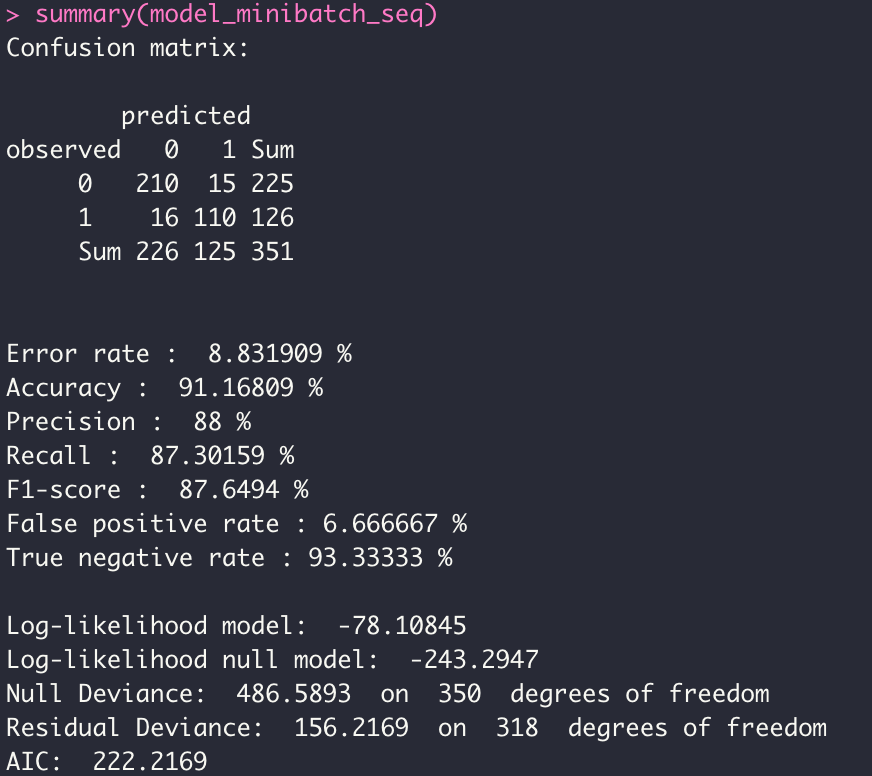
- MINI BATCH MODE
model_minibatch_seq <- dgrglm.fit(y~., data = data, mode_compute="sequentiel",
                       leaning_rate=0.1, max_iter=2000,tolerance=1e-06,batch_size = 10)
summary(model_minibatch_seq)
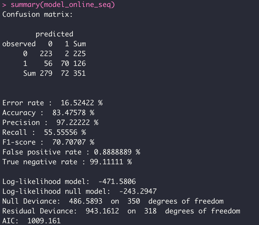
- ONLINE MODE
model_online_seq <- dgrglm.fit(y~., data = data, mode_compute="sequentiel",leaning_rate=0.1,
                               max_iter=1000,tolerance=1e-06, batch_size = 1)
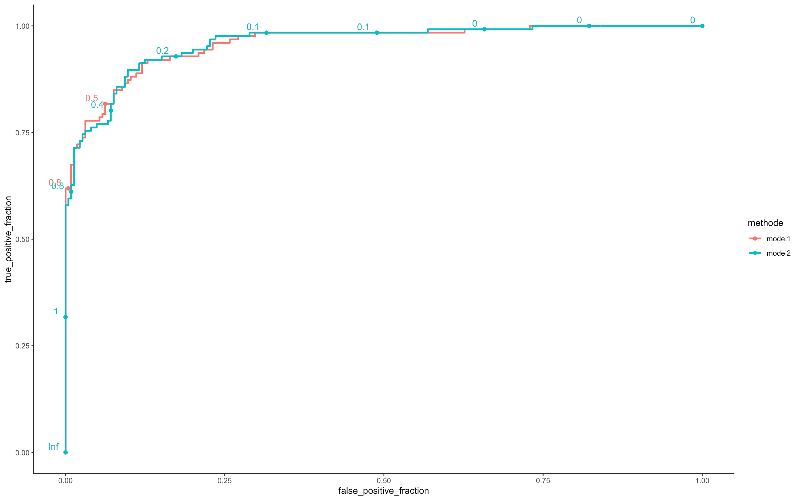
In order to test our different models, we have developed an external function, which displays the ROC curves according to the probabilities of each model. This function is in the trace file devtools_history.R
perf <- compare_model(probas_mod1=model_batch_seq$probas,
                      probas_mod2=model_minibatch_seq$probas,
                      y=model_minibatch_seq$y_val[,1])
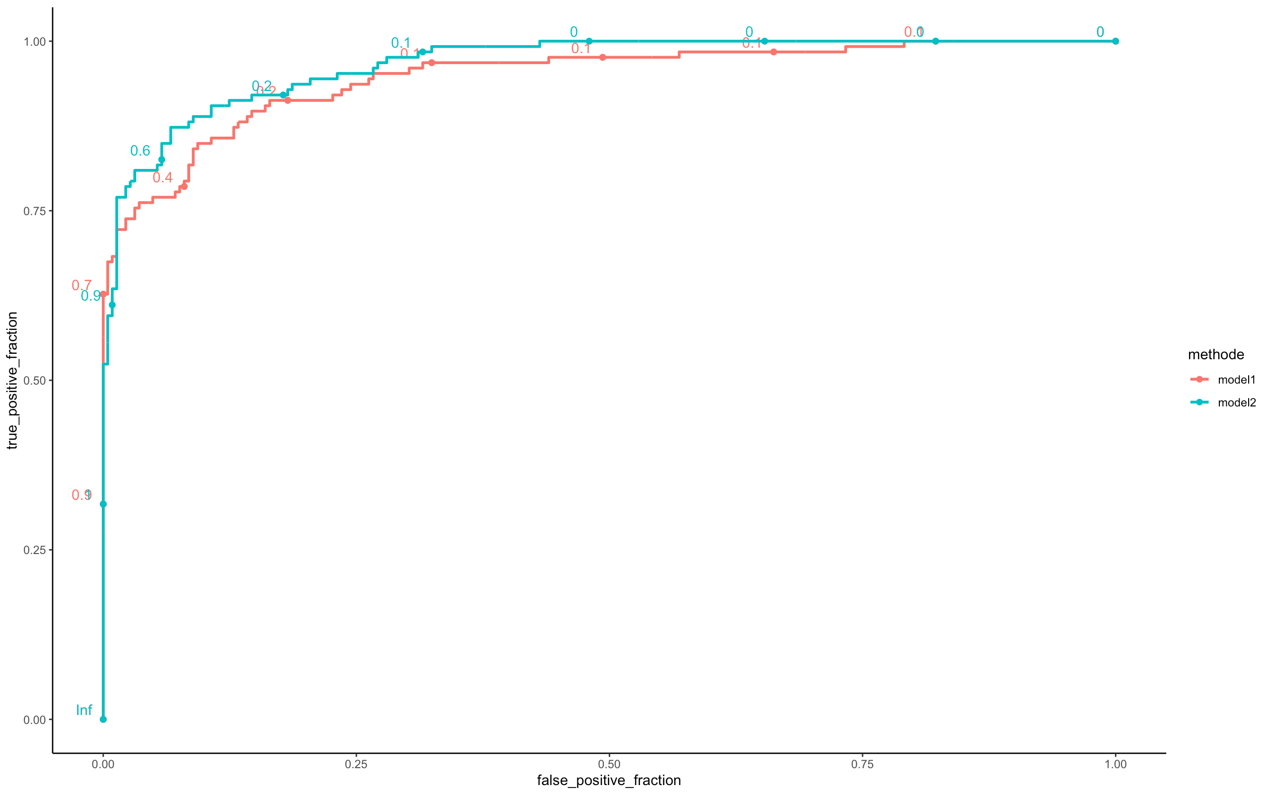
In terms of their ROC curves, the two models are roughly similar in terms of predictions. In terms of their ROC curves, the two models are roughly similar in terms of predictions. Nevertheless model 2 is better.
perf <- compare_model(probas_mod1=model_batch_seq$probas,
probas_mod2=model_online_seq$probas,
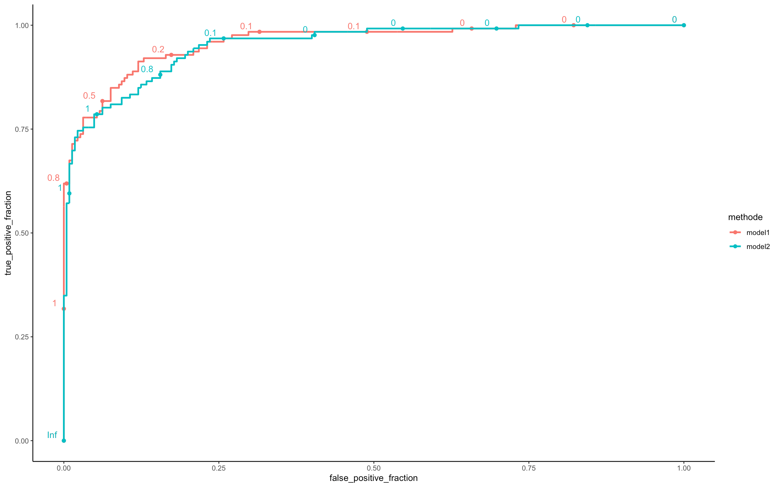
y=model_online_seq$y_val[,1])
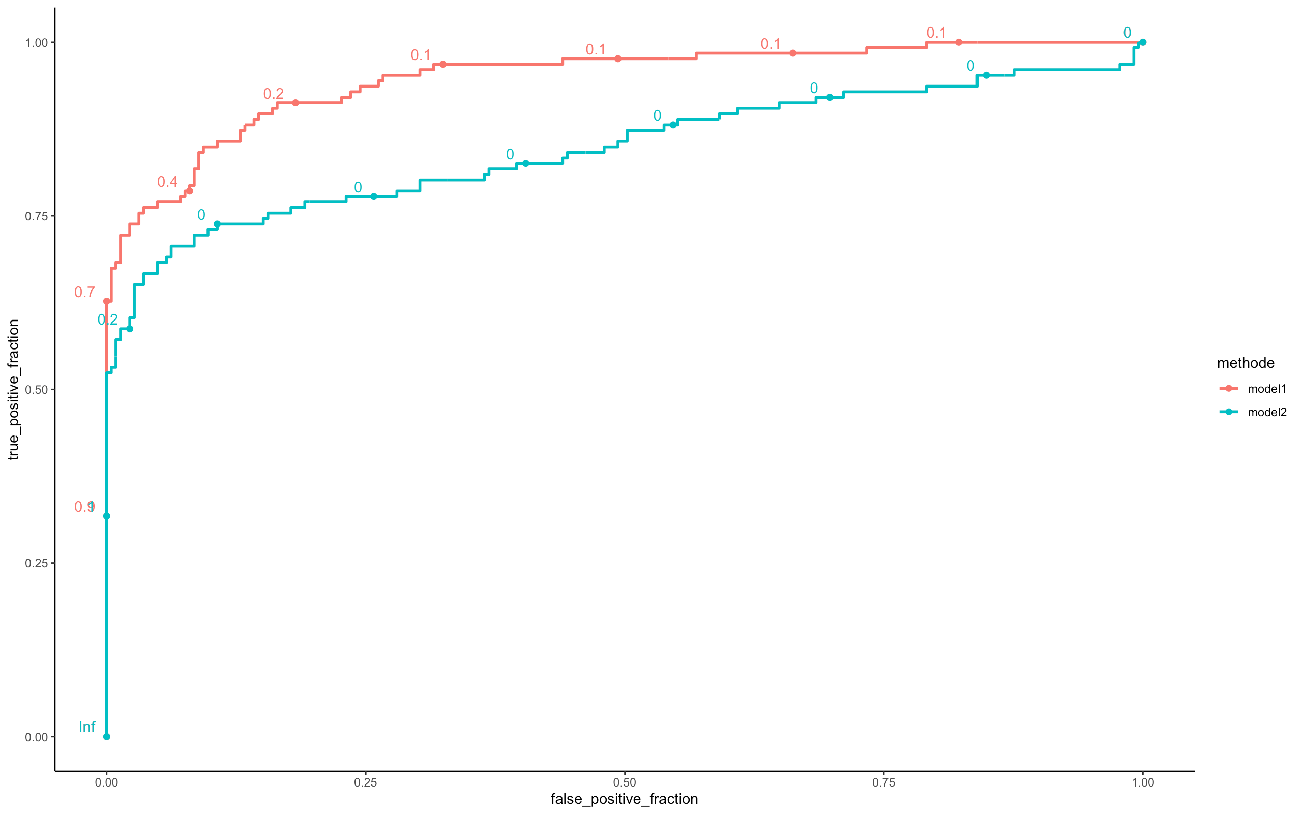
Here we see that the Batch model is clearly better than the online model in terms of prediction
parallel execution:
The idea of parallel execution is to slice the data according to the number of cores of the machine and to distribute the calculations on these cores. If the user provides a number of cores not available, the program automatically chooses the max-1 cores.
For a parallel execution, specify comput_mode ='parallel' and nbcores=max-1 in your computer.
- Mode BATCH
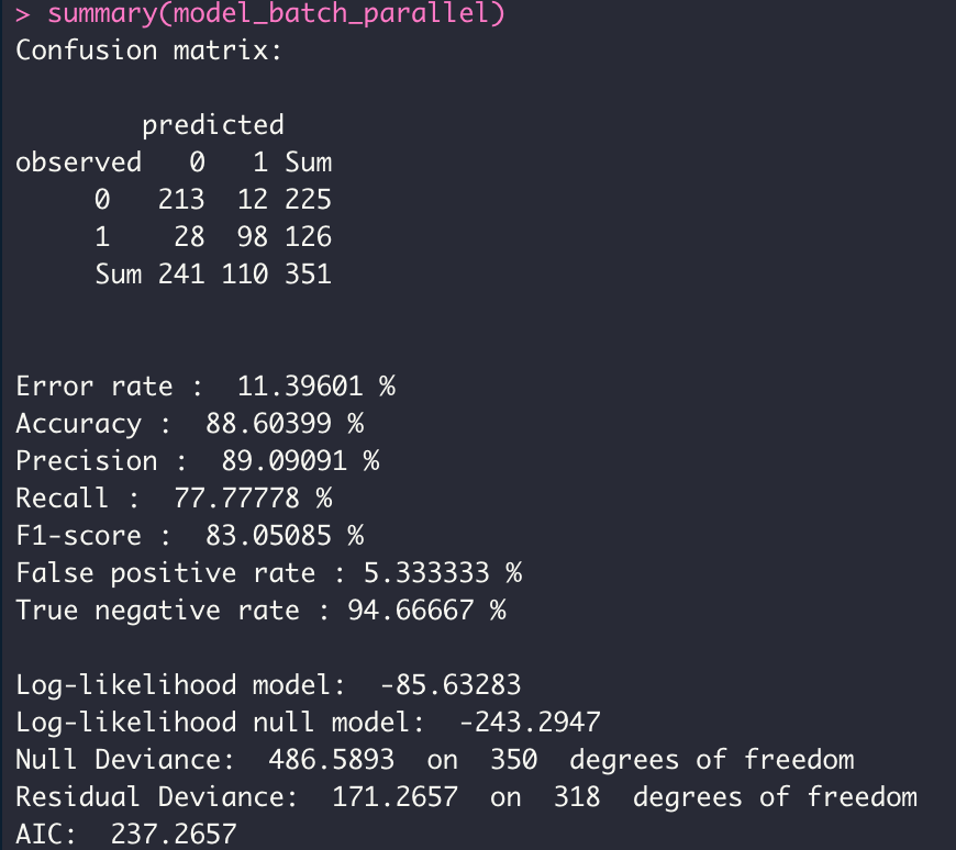
model_batch_parallel <- dgrglm.fit(y~., data = data, ncores=3, mode_compute="parallel",
                                   leaning_rate=0.1, max_iter=1000,tolerance=1e-06)
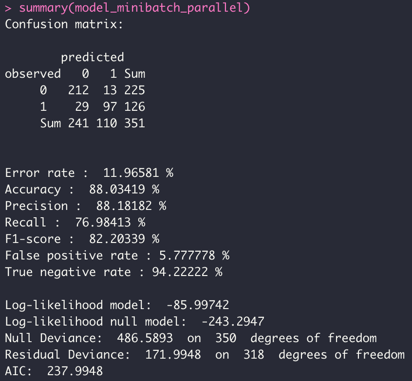
- MODE MINI BATCH
model_minibatch_parallel <- dgrglm.fit(y~., data = data, ncores=3, mode_compute="parallel",
                                       leaning_rate=0.1, max_iter=1000,tolerance=1e-06,
                                       batch_size = 10)
- MODE ONLINE
model_online_parallel <- dgrglm.fit(y~., data = data, ncores=3, mode_compute="parallel",
                                    leaning_rate=0.1, max_iter=1000,tolerance=1e-06,
                                    batch_size = 1)
perf <- compare_model(probas_mod1=model_batch_parallel$probas,
                      probas_mod2=model_minibatch_parallel$probas,
                      y=model_minibatch_parallel$y_val[,1])

perf <- compare_model(probas_mod1=model_batch_parallel$probas,
                      probas_mod2=model_online_parallel$probas,
                      y=model_online_parallel$y_val[,1])

perf <- compare_model(probas_mod1=model_minibatch_parallel$probas,
                      probas_mod2=model_online_parallel$probas,
                      y=model_online_parallel$y_val[,1])

Looking at the three ROC curves, we can assume that the 03 models (Batch, Mini Batch, Online) are similar in terms of predictions. However there is a big difference on the execution time (see Microbenchmark).
Microbenchmark
- Sequential
library(microbenchmark)
microbenchmark(
  model_batch_seq <- dgrglm.fit(y~., data = data, mode_compute="sequentiel",
                                leaning_rate=0.1, max_iter=1000,tolerance=1e-06),
  model_minibatch_seq <- dgrglm.fit(y~., data = data, mode_compute="sequentiel",leaning_rate=0.1,
                                    max_iter=1000,tolerance=1e-06,batch_size = 10),
  model_online_seq <- dgrglm.fit(y~., data = data, mode_compute="sequentiel",
                                 leaning_rate=0.1, max_iter=1000,tolerance=1e-06, batch_size = 1),
  times = 1,
  unit = "s"
)
- Parallel
microbenchmark(
  model_batch_parallel <- dgrglm.fit(y~., data = data, ncores=3, mode_compute="parallel",
                                     leaning_rate=0.1, max_iter=1000,tolerance=1e-06),
  model_minibatch_parallel <- dgrglm.fit(y~., data = data, ncores=3, mode_compute="parallel",
                                         leaning_rate=0.1, max_iter=1000,tolerance=1e-06,batch_size = 10),
  model_online_parallel <- dgrglm.fit(y~., data = data, ncores=3, mode_compute="parallel",
                                      leaning_rate=0.1, max_iter=1000,tolerance=1e-06,batch_size = 1),
  times = 1,
  unit = "s"
)
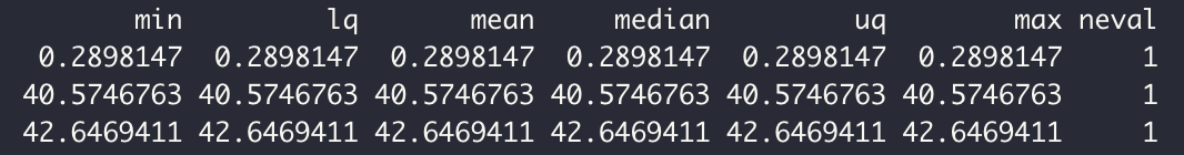
We implemented logistic regression in sequential and parallel mode. The idea was to see if using all the computational cores a machine has for the execution of the algorithm could increase the speed or not.
According to the results of the Benchmark, there does not seem to be a global gain by executing in parallel (cutting data in lines) as opposed to a sequential execution
To verify this hypothesis we will generate logistic data manually and play on the number of individuals and variables and test for each case the computation time.
Logistic data generation
set.seed(103)
n <-1000000  # Number of obervations
p <- 5 # Number of variables
theta = runif(p+1) # Theta vector
X <- cbind(1,matrix(rnorm(n*p),n,p))
Z <- X %*% theta # linear combination of variables
fprob <- ifelse(Z<0, exp(Z)/(1+exp(Z)),1/(1+exp(-Z))) # Calcul des probas d'affectation
y<- rbinom(n,1,fprob)
data = as.data.frame(cbind(X,y))
data$V1 <- NULL # delete colomn de biais. It will be created when fit is called
The dataset is well generated. It contains 1 million rows
In the following we will just play on n and p to increase or decrease the number of variables and/or individuals. Now, Let's run the Microbenchmark again on the set of :
case n=200 rows and p=400 variables.
- Sequential
- Parallel
case n=10000 rows and p=5 variables.
- Sequential
- Parallel
After several combinations of n and p, we see that the sequential always wins over the parallel. But this seems logical because of:
- the number and size of messages exchanged between workers and the master;
- the size of the task which will be evaluated several times (n iterations);
- how much data must be sent between the communicating entities;
- etc.
Features Selection
- feature_selection=TRUE, p_value=0.01
We have the possibility to create the model on variables selected automatically according to their relevance.
 model_batch_parallel <- dgrglm.fit(y~., data = data, ncores=3, mode_compute="parallel",
                                    leaning_rate=0.1, max_iter=1000,tolerance=1e-06,
                                    feature_selection=TRUE, p_value=0.01)
Centering reduction
- centering = TRUE
model_batch_parallel <- dgrglm.fit(y~., data = data, ncores=3, mode_compute="parallel",
                                  leaning_rate=0.1,max_iter=1000,tolerance=1e-06,
                                  feature_selection=TRUE, p_value=0.01,
                                  centering = TRUE)
Elasticnet
- iselasticnet=TRUE, rho=0.1, C=0.1
model_batch_parallel <- dgrglm.fit(y~., data = data, ncores=3, mode_compute="parallel",leaning_rate=0.1,
                                   max_iter=1000, tolerance=1e-06,
                                   feature_selection=TRUE, p_value=0.01,
                                   centering = FALSE,
                                   iselasticnet=TRUE, rho=0.1, C=0.1)
- si rho=0 ===> RIDGE
- si rho=1 ===> LASSO
2. Multinomiale regression
- For multiclass regression the target variable is coded in binary (One vs ALL).
dgrglm.multiclass.fit(formule, data, leaning_rate=0.1, max_iter=3000, tolerance=1e-04,
                      random_state=102, centering = FALSE){...}
Beuleup93/dgrGlm documentation built on Dec. 17, 2021, 10:50 a.m.
R Package Documentation
Browse R Packages
We want your feedback!
Note that we can't provide technical support on individual packages. You should contact the package authors for that.
dgrGlm: GRadient Descent For Logistic Regression
DESCRIPTION
This project is part of our training in Data Science at the University of Lyon 2. The main objective is to develop an R package under S3 that allows to do binary logistic regression distributed on the different cores of the user's computer. Gradient descent is used for the optimization of the parameters. Here the idea is to allow the user to take advantage of the totality of these computer resources, if of course this can help to make the execution of the calculations faster. Here are the different functionalities of our package that we will present in the following lines:
- Binary logistic regression model in sequential mode
- Splitting of calculations and data for parallel execution
- Binary logistic regression model in parallel mode
- Comparison of model predictions
- Automatic Features selection
- Model Microbenchmark
- Elasticnet (Ridge and Lasso)
- Multinomiale logistic regression
- Recoding of the target variable (One vs All)
Logistic Regression
Logistic regression is an old and well-known statistical predictive method that applies to binary classification, but can be easily extended to the multiclass framework (multinomial regression in particular, but not only...).It has become popular in recent years in machine learning thanks to "new" computational algorithms (optimization) and powerful libraries. The work on regularization makes its use efficient in the context of high dimensional learning (nb. Var. Expl. >> nb. Obsv.). It is related to neural networks (simple perceptron). The objective of this guide is not to explain the mathematical formulas around logistic regression but to give you an overview of our package.
Installation and data loading
In order to use our package, you should install it from Github.
library(devtools)
install_github("Beuleup93/dgrGlm")
Once the package is downloaded and successfully installed, please load it for use.
library(dgrGlm)
Now you can access all available functions of the package. To prove it, we will display the documentation of our fit function. you can write in your console: ?dgrGlm.fit to see the documentation or:
help(dgrGlm.fit)
In order to test our functions, we will work with the dataset ionosphere.xlsx. It consists of 351 obervations and 34 variables.
1. Binary Logistic Regression
We will start by testing the binary logistic regression on our dataset. The variable to be explained is Y and the explicatives variables are a03,...,a34.
General function fit
dgrglm.fit <- function(formule, data, ncores=NA, mode_compute="parallel", leaning_rate=0.1,
max_iter=100, tolerance=1e-04, batch_size=NA,
random_state=102, centering = FALSE, feature_selection=FALSE,
p_value=0.01, rho=0.1, C=0.1, iselasticnet=FALSE){...}
This function takes into account several aspects: - sequential execution with mode_compute="sequentiel" - parallel execution with for example ncores=4, and mode_compute="parallel" - Execution in Batch, Mini Batch and Online modes with batch_size=NA - Centering reduction of explanatory variables with centering = TRUE - Selection of variables by playing on the arguments feature_selection=TRUE, p_value=0.01 - Elasticnet (Ridge for rho=0 and Lasso for rho=1) avec les arguments C et rho. For each algorithm the principle is explained in the report.
sequential execution:
For a sequential execution, specify comput_mode ='sequentiel'.
- BATCH Mode
model_batch_seq <- dgrglm.fit(y~., data = data, mode_compute="sequentiel",
leaning_rate=0.1, max_iter=1000,tolerance=1e-06)
summary(model_batch_seq)
We have overloaded the print and summary methods for a display adapted to our objects returned by fit.
- MINI BATCH MODE
model_minibatch_seq <- dgrglm.fit(y~., data = data, mode_compute="sequentiel",
leaning_rate=0.1, max_iter=2000,tolerance=1e-06,batch_size = 10)
summary(model_minibatch_seq)
- ONLINE MODE
model_online_seq <- dgrglm.fit(y~., data = data, mode_compute="sequentiel",leaning_rate=0.1,
max_iter=1000,tolerance=1e-06, batch_size = 1)
In order to test our different models, we have developed an external function, which displays the ROC curves according to the probabilities of each model. This function is in the trace file devtools_history.R
perf <- compare_model(probas_mod1=model_batch_seq$probas,
probas_mod2=model_minibatch_seq$probas,
y=model_minibatch_seq$y_val[,1])
In terms of their ROC curves, the two models are roughly similar in terms of predictions. In terms of their ROC curves, the two models are roughly similar in terms of predictions. Nevertheless model 2 is better.
perf <- compare_model(probas_mod1=model_batch_seq$probas,
probas_mod2=model_online_seq$probas,
y=model_online_seq$y_val[,1])
Here we see that the Batch model is clearly better than the online model in terms of prediction
parallel execution:
The idea of parallel execution is to slice the data according to the number of cores of the machine and to distribute the calculations on these cores. If the user provides a number of cores not available, the program automatically chooses the max-1 cores.
For a parallel execution, specify comput_mode ='parallel' and nbcores=max-1 in your computer.
- Mode BATCH
model_batch_parallel <- dgrglm.fit(y~., data = data, ncores=3, mode_compute="parallel",
leaning_rate=0.1, max_iter=1000,tolerance=1e-06)
- MODE MINI BATCH
model_minibatch_parallel <- dgrglm.fit(y~., data = data, ncores=3, mode_compute="parallel",
leaning_rate=0.1, max_iter=1000,tolerance=1e-06,
batch_size = 10)
- MODE ONLINE
model_online_parallel <- dgrglm.fit(y~., data = data, ncores=3, mode_compute="parallel",
leaning_rate=0.1, max_iter=1000,tolerance=1e-06,
batch_size = 1)
perf <- compare_model(probas_mod1=model_batch_parallel$probas,
probas_mod2=model_minibatch_parallel$probas,
y=model_minibatch_parallel$y_val[,1])
perf <- compare_model(probas_mod1=model_batch_parallel$probas,
probas_mod2=model_online_parallel$probas,
y=model_online_parallel$y_val[,1])
perf <- compare_model(probas_mod1=model_minibatch_parallel$probas,
probas_mod2=model_online_parallel$probas,
y=model_online_parallel$y_val[,1])
Looking at the three ROC curves, we can assume that the 03 models (Batch, Mini Batch, Online) are similar in terms of predictions. However there is a big difference on the execution time (see Microbenchmark).
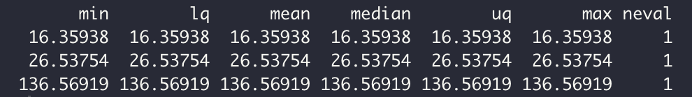
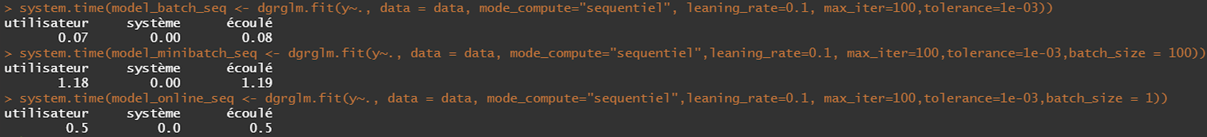
Microbenchmark
- Sequential
library(microbenchmark)
microbenchmark(
model_batch_seq <- dgrglm.fit(y~., data = data, mode_compute="sequentiel",
leaning_rate=0.1, max_iter=1000,tolerance=1e-06),
model_minibatch_seq <- dgrglm.fit(y~., data = data, mode_compute="sequentiel",leaning_rate=0.1,
max_iter=1000,tolerance=1e-06,batch_size = 10),
model_online_seq <- dgrglm.fit(y~., data = data, mode_compute="sequentiel",
leaning_rate=0.1, max_iter=1000,tolerance=1e-06, batch_size = 1),
times = 1,
unit = "s"
)
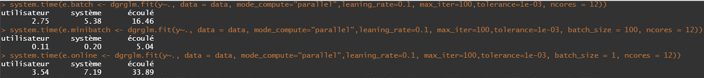
- Parallel
microbenchmark(
model_batch_parallel <- dgrglm.fit(y~., data = data, ncores=3, mode_compute="parallel",
leaning_rate=0.1, max_iter=1000,tolerance=1e-06),
model_minibatch_parallel <- dgrglm.fit(y~., data = data, ncores=3, mode_compute="parallel",
leaning_rate=0.1, max_iter=1000,tolerance=1e-06,batch_size = 10),
model_online_parallel <- dgrglm.fit(y~., data = data, ncores=3, mode_compute="parallel",
leaning_rate=0.1, max_iter=1000,tolerance=1e-06,batch_size = 1),
times = 1,
unit = "s"
)
We implemented logistic regression in sequential and parallel mode. The idea was to see if using all the computational cores a machine has for the execution of the algorithm could increase the speed or not. According to the results of the Benchmark, there does not seem to be a global gain by executing in parallel (cutting data in lines) as opposed to a sequential execution
To verify this hypothesis we will generate logistic data manually and play on the number of individuals and variables and test for each case the computation time.
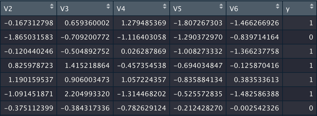
Logistic data generation
set.seed(103)
n <-1000000 # Number of obervations
p <- 5 # Number of variables
theta = runif(p+1) # Theta vector
X <- cbind(1,matrix(rnorm(n*p),n,p))
Z <- X %*% theta # linear combination of variables
fprob <- ifelse(Z<0, exp(Z)/(1+exp(Z)),1/(1+exp(-Z))) # Calcul des probas d'affectation
y<- rbinom(n,1,fprob)
data = as.data.frame(cbind(X,y))
data$V1 <- NULL # delete colomn de biais. It will be created when fit is called
The dataset is well generated. It contains 1 million rows
In the following we will just play on n and p to increase or decrease the number of variables and/or individuals. Now, Let's run the Microbenchmark again on the set of :
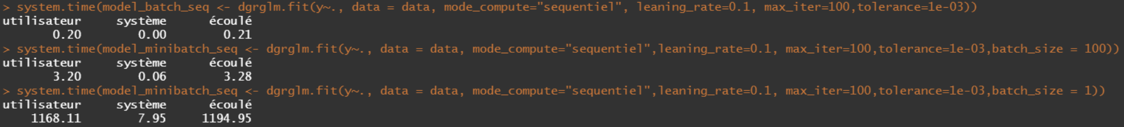
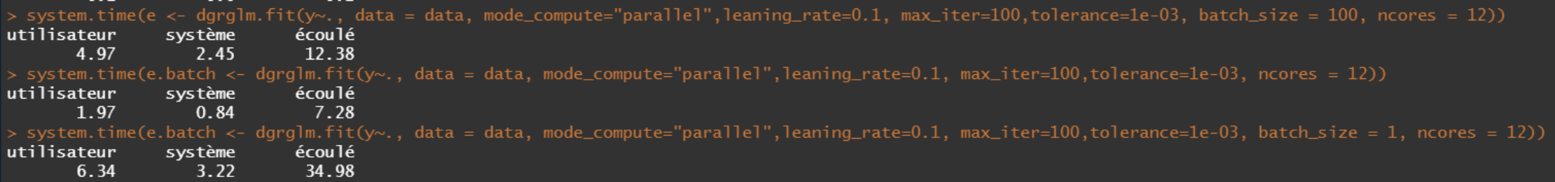
case n=200 rows and p=400 variables.
- Sequential
- Parallel
case n=10000 rows and p=5 variables.
- Sequential
- Parallel
After several combinations of n and p, we see that the sequential always wins over the parallel. But this seems logical because of: - the number and size of messages exchanged between workers and the master; - the size of the task which will be evaluated several times (n iterations); - how much data must be sent between the communicating entities; - etc.
Features Selection
- feature_selection=TRUE, p_value=0.01
We have the possibility to create the model on variables selected automatically according to their relevance.
model_batch_parallel <- dgrglm.fit(y~., data = data, ncores=3, mode_compute="parallel",
leaning_rate=0.1, max_iter=1000,tolerance=1e-06,
feature_selection=TRUE, p_value=0.01)
Centering reduction
- centering = TRUE
model_batch_parallel <- dgrglm.fit(y~., data = data, ncores=3, mode_compute="parallel",
leaning_rate=0.1,max_iter=1000,tolerance=1e-06,
feature_selection=TRUE, p_value=0.01,
centering = TRUE)
Elasticnet
- iselasticnet=TRUE, rho=0.1, C=0.1
model_batch_parallel <- dgrglm.fit(y~., data = data, ncores=3, mode_compute="parallel",leaning_rate=0.1,
max_iter=1000, tolerance=1e-06,
feature_selection=TRUE, p_value=0.01,
centering = FALSE,
iselasticnet=TRUE, rho=0.1, C=0.1)
- si rho=0 ===> RIDGE
- si rho=1 ===> LASSO
2. Multinomiale regression
- For multiclass regression the target variable is coded in binary (One vs ALL).
dgrglm.multiclass.fit(formule, data, leaning_rate=0.1, max_iter=3000, tolerance=1e-04,
random_state=102, centering = FALSE){...}
R Package Documentation
Browse R Packages
We want your feedback!
Note that we can't provide technical support on individual packages. You should contact the package authors for that.
Embedding an R snippet on your website
Add the following code to your website.
For more information on customizing the embed code, read Embedding Snippets.