In GOVS-pack/GOVS: Genome optimization via virtual simulation

require(GOVS)
knitr::opts_chunk$set(
  collapse = TRUE,
  comment = "#>"
)

Contents {#contents}

1. Package installation
2. Data preparation a. Genotypic data b. Phenotypic data c. Bins data d. Bins information data
3. Genome Optimization via Virtual Simulation
4. rrBLUP for Genotype-to-phenotype prediciton
5. Construct bin map
6. Visualization of bin a. Plot bin map b. Plot mosaic plot

This vignette briefly introduces some typical examples of GOVS to help users get started quickly. Detailes and other functions of GOVS,please see Tutorial for GOVS or Reference Manual.

Homepage: https://govs-pack.github.io/

Github repository: https://github.com/GOVS-pack/GOVS

How to install GOVS {#Installation}

1. Github install

## install dependencies and GOVS
install.packages(c("ggplot2","rrBLUP","lsmeans","readr","pbapply","pheatmap","emmeas"))
require("devtools")
install_github("GOVS-pack/GOVS") 
## if you want build vignette in GOVS 
install_github("GOVS-pack/GOVS",build_vignettes = TRUE)

2. Download .tar.gz package and install

Download link: https://github.com/GOVS-pack/GOVS/raw/master/GOVS_1.0.tar.gz

## install dependencies and GOVS with bult-in vignette
install.packages(c("ggplot2","rrBLUP","lsmeans","readr","pbapply","pheatmap","emmeas"))
install.packages("DownloadPath/GOVS_1.0.tar.gz")

Library GOVS

library("GOVS")

Back to Contents

Input data for GOVS {#data_preparation}

Genotypic data (hapmap format, matrix) {#G}

SNP rs must coded with pattern "chr[0-9].s/_[0-9]*" (eg: chr1.s_4831, "1" for chromosome, "4831" for locus).

data(MZ)
MZ[1:10,1:15]

Phenotypic data {#P}

Phenotypic data (dataframe), first column is lines ID.

data(phe)
head(phe)

Bins data {#bins}

Bins data (matrix), each row represents a bin (reconbination fragment) and each column represents a progeny, contents represent the origins of the bins tracing back to the parental lines.

data(bins)
bins[1:5,1:5]

Bins information data {#binsInfo}

Bins information data (dataframe) corresponding to bins data, consists of five columns (bin ID, chromsome, start position, end position and length of each bin).

data("binsInfo")
head(binsInfo)

NOTE: The header of bins, the first column of phenotype and the header of genotype must be unified, we recommend unify these ID with patrental ID.

Back to Contents

Run GOVS {#GOVS}

GOVS_res <- GOVS(MZ,pheno = phe,trait = "EW",which = "max",bins = bins,
                 binsInfo = binsInfo,module = "DES")

Output of GOVS:

A list containing the following elements (if output = NULL, default NULL) or several files with same prefix (if output is defined).

• $GORes Genome optimization results.
• $virtualGenome A matrix involves of three optimal virtual genomes.
• $statRes A data frame regarding statistics results of virtual simulation.
  • Lines Lines
  • Bins(#) The number (#) of bins that a line contributed to the simulated genome.
  • Bins(%) The number of bins that a line contributed accounting for the proportion (%) of simulated genome.
  • Fragments(%) The total length of genomic fragments that a line contributed accounting for the proportion (%) of simulated genome.
  • phenotype The phenotypic value of the corresponding lines or their offspring.
  • phenotypeRank The phenotype rank.
  • Cumulative(%) The cumulative percentage of fragments contributing to the simulated genome.
    

GOVS_res$statRes

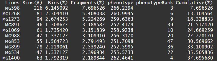
Figure1 Statistic summary of GOVS

Genotytpe-to-phenotype prediciton (rrBLUP) {#G2P}

This function performs genotpye-to-phenotype prediciton via ridge regression best linear unbiased prediction (rrBLUP) model (Endelman, 2011). The inputs is genotypeic data.

## load hapmap data (genomic data) of MZ hybrids
data(MZ)
## load phenotypic data of MZ hybrids
data(phe)
## pre-process for G2P prediction 
rownames(MZ) <- MZ[,1]
MZ <- MZ[,-c(1:11)]
MZ.t <- t(MZ)
## conversion
MZ.n <- transHapmap2numeric(MZ.t)
dim(MZ.t)
## prediction
idx1 <- sample(1:1404,1000)
idx2 <- setdiff(1:1404,idx1)
predRes <- SNPrrBLUP(MZ.n,phe$EW,idx1,idx2,fix = NULL,model = FALSE)

head(predRes)

## scatter plot 
plot(phe$EW[idx2],predRes,xlab = "Observed value", ylab =  "Predicted value")

Figure2 Observed value VS predicted value

Back to Contents

Construct bin map {#binmap}

IBD map was constructed of contributions from the parents onto the progeny lines discribed by Liu et al. (Liu et al., 2020) based hidden Markov model (HMM) (Mott et al, 2000). Here we take chromosome-10 of one offspring as an example.

## load example data
data(IBDTestData)

## compute rou from genetic position
rou = IBDTestData$posGenetic
rou = diff(rou)
rou = ifelse(rou<0,0,rou)

## constract IBD map of chr10 for one progeny
IBDRes <- IBDConstruct(snpParents = IBDTestData$snpParents,
markerInfo = IBDTestData$markerInfo,
snpProgeny = IBDTestData$snpProgeny,q = 0.97,G = 9,rou = rou)

Output of IBDConstruct:

A list regarding constructed bin map.

• bin Results of IBD analysis, each row represents a bin fragment.
• binsInfo Data frame, including bins index, start, end, length of bins locus.

Back to Contents

Visualization of bin map {#plotmap}

Plot IBD bin map for one progeny {#plotbin}

## load example data
data(IBDTestData)

## compute rou from genetic position
rou = IBDTestData$posGenetic
rou = diff(rou)
rou = ifelse(rou<0,0,rou)

## constract IBD map of chr10 for one progeny
IBDRes <- IBDConstruct(snpParents = IBDTestData$snpParents,
markerInfo = IBDTestData$markerInfo,
snpProgeny = IBDTestData$snpProgeny,q = 0.97,G = 9,rou = rou)

## plot
# color
color <- c("#DA053F","#FC0393","#C50F84","#D870D4","#DCA0DC","#4A0380",
           "#9271D9","#0414FB","#2792FC","#4883B2","#2CFFFE","#138B8A",
           "#42B373","#9BFB9C","#84FF2F","#566B32","#FED62D","#FD8A21",
           "#F87E75","#B01D26","#7E0006","#A9A9A9","#FFFE34","#FEBFCB")
names(color) <- 1:24

# parent label
parentInfo <- c("5237","E28","Q1261","CHANG7-2","DAN340","HUANGC","HYS",
                "HZS","TY4","ZI330","ZONG3","LX9801","XI502","81515",
                "F349","H21","JI853","JI53","LV28","YUANFH","SHUANG741",
                "K12","NX110","ZONG31")
names(parentInfo) <- 1:24

# plot
binsPlot(IBDRes,color,parentInfo,24)

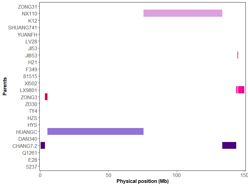
Figure3 Bins map plot

Visualization of overall bins data {#mosaic}

Take chromosome-1 and first 200 progeny as an example.

## load data
data(bins)
data(binsInfo)
## color
color <- c("#DA053F","#FC0393","#C50F84","#D870D4","#DCA0DC","#4A0380",
            "#9271D9","#0414FB","#2792FC","#4883B2","#2CFFFE","#138B8A",
            "#42B373","#9BFB9C","#84FF2F","#566B32","#FED62D","#FD8A21",
            "#F87E75","#B01D26","#7E0006","#A9A9A9","#FFFE34","#FEBFCB")

mosaicPlot(bins = bins,binsInfo = binsInfo,chr = 1,resolution = 500,
                  color = color,
                  list = colnames(bins)[1:200])

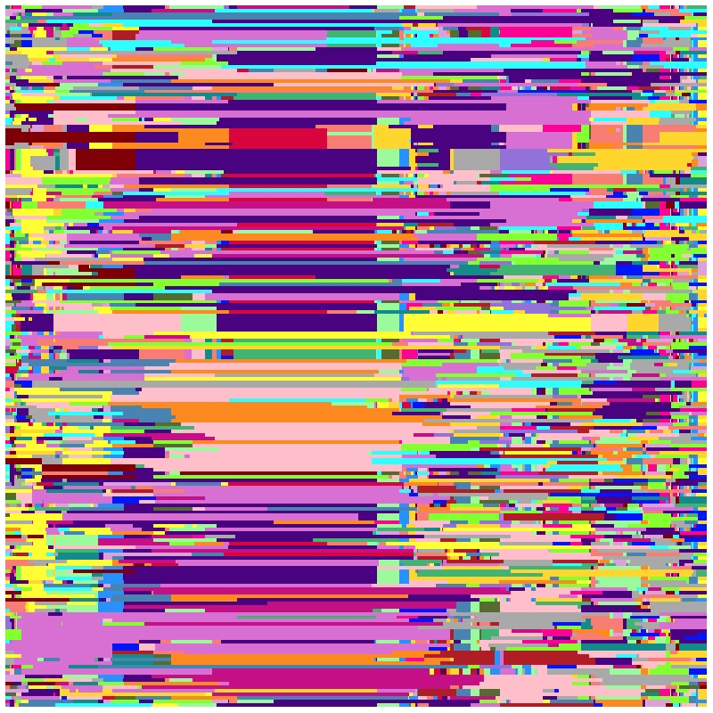
Figure4 Bins mosaic plot

Back to Contents

References {#reference}

Endelman, J. B. (2011). Ridge regression and other kernels for genomic selection with R package rrBLUP. The plant genome, 4(3) https://doi.org/10.3835/plantgenome2011.08.0024

Mott, R., Talbot, C. J., Turri, M. G., Collins, A. C., & Flint, J. (2000). A method for fine mapping quantitative trait loci in outbred animal stocks. Proceedings of the National Academy of Sciences, 97(23), 12649-12654. https://doi.org/10.1073/pnas.230304397

Liu H J, Wang X, Xiao Y, et al. (2020) CUBIC: an atlas of genetic architecture promises directed maize improvement[J]. Genome biology, 21(1): 1-17. https://doi.org/10.1186/s13059-020-1930-x

Back to Contents

GOVS-pack/GOVS documentation built on Oct. 9, 2022, 8:29 a.m.