In LieberInstitute/spatialLIBD: spatialLIBD: an R/Bioconductor package to visualize spatially-resolved transcriptomics data
knitr::opts_chunk$set(
    collapse = TRUE,
    comment = "#>",
    fig.path = "man/figures/README-",
    out.width = "100%"
)
spatialLIBD 


Welcome to the spatialLIBD project! It is composed of:
- a shiny web application that we are hosting at spatial.libd.org/spatialLIBD/ that can handle a limited set of concurrent users,
- a Bioconductor package at bioconductor.org/packages/spatialLIBD (or from here) that lets you analyze the data and run a local version of our web application (with our data or yours),
- and a research article with the scientific knowledge we drew from this dataset. The analysis code for our project is available here and the high quality figures for the manuscript are available through Figshare.
The web application allows you to browse the LIBD human dorsolateral pre-frontal cortex (DLPFC) spatial transcriptomics data generated with the 10x Genomics Visium platform. Through the R/Bioconductor package you can also download the data as well as visualize your own datasets using this web application. Please check the manuscript or bioRxiv pre-print for more details about this project.
If you write about this website, the data or the R package please use
the #spatialLIBD hashtag. See previous tagged Bluesky posts
here.
Thank you!
Study design
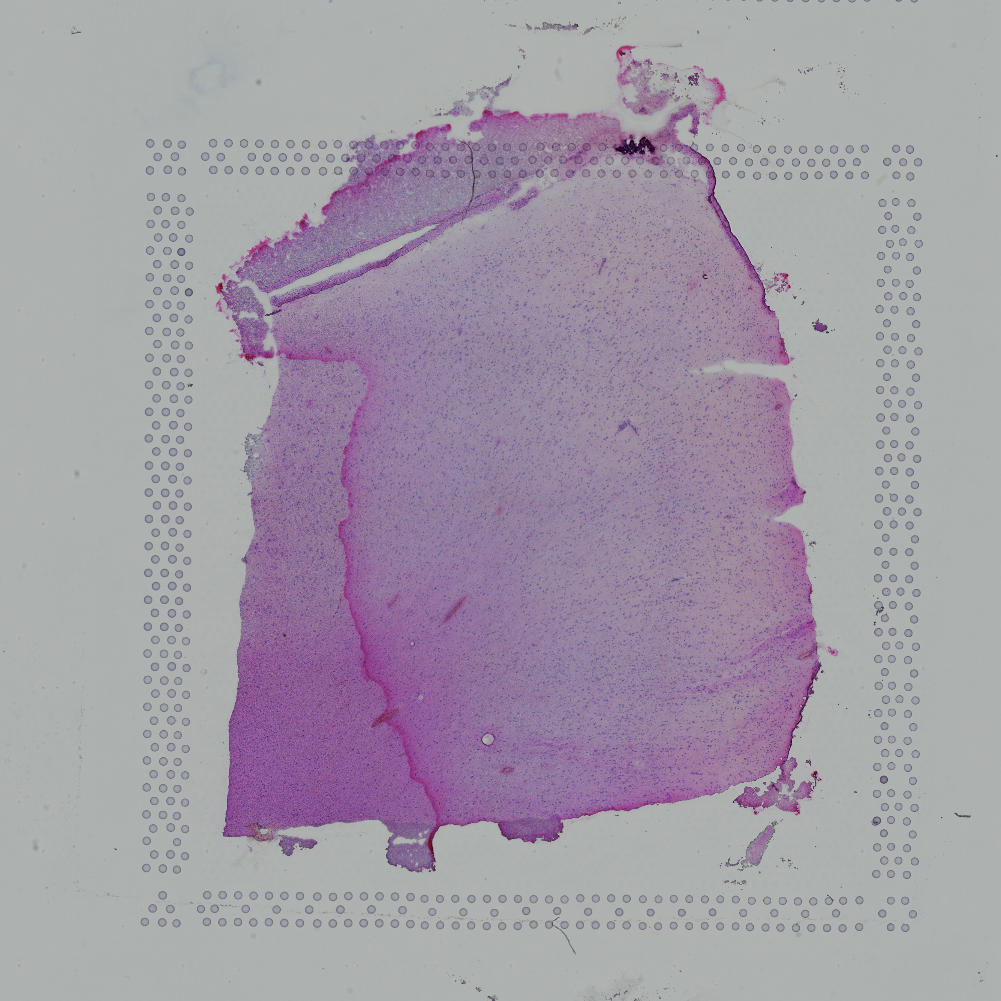
As a quick overview, the data presented here is from portion of the DLPFC that spans six neuronal layers plus white matter (A) for a total of three subjects with two pairs of spatially adjacent replicates (B). Each dissection of DLPFC was designed to span all six layers plus white matter (C). Using this web application you can explore the expression of known genes such as SNAP25 (D, a neuronal gene), MOBP (E, an oligodendrocyte gene), and known layer markers from mouse studies such as PCP4 (F, a known layer 5 marker gene).

This web application was built such that we could annotate the spots to layers as you can see under the spot-level data tab. Once we annotated each spot to a layer, we compressed the information by a pseudo-bulking approach into layer-level data. We then analyzed the expression through a set of models whose results you can also explore through this web application. Finally, you can upload your own gene sets of interest as well as layer enrichment statistics and compare them with our LIBD Human DLPFC Visium dataset.
If you are interested in running this web application locally, you can do so thanks to the spatialLIBD R/Bioconductor package that powers this web application as shown below.
## Run this web application locally
spatialLIBD::run_app()

## You will have more control about the length of the
## session and memory usage.

## You could also use this function to visualize your
## own data given some requirements described
## in detail in the package vignette documentation
## at http://research.libd.org/spatialLIBD/.
Shiny website mirrors
- Main shiny application website (note that the link must have a trailing slash
/ for it to work)
- Shinyapps This version has less RAM memory but is typically deployed using the latest version of
spatialLIBD.
Introductory material
If you prefer to watch a video overview of the HumanPilot project, check the following journal club presentation of the main results.
You might also be interested in the explainer video and companion blog post as well as the original Feb 29, 2020 blog post from when we first made this project public.
R/Bioconductor package
The spatialLIBD package contains functions for:
- Accessing the spatial transcriptomics data from the LIBD Human Pilot project (code on GitHub) generated with the Visium platform from 10x Genomics. The data is retrieved from Bioconductor's
ExperimentHub.
- Visualizing the spot-level spatial gene expression data and clusters.
- Inspecting the data interactively either on your computer or through spatial.libd.org/spatialLIBD/.
For more details, please check the documentation website or the Bioconductor package landing page here.
Installation instructions
Get the latest stable R release from CRAN. Then install spatialLIBD from Bioconductor using the following code:
if (!requireNamespace("BiocManager", quietly = TRUE)) {
    install.packages("BiocManager")
}

BiocManager::install("spatialLIBD")
If you want to use the development version of spatialLIBD, you will need to use the R version corresponding to the current Bioconductor-devel branch as described in more detail on the Bioconductor website. Then you can install spatialLIBD from GitHub using the following command.
BiocManager::install("LieberInstitute/spatialLIBD")
Access the data
Through the spatialLIBD package you can access the processed data in it's final R format. However, we also provide a table of links so you can download the raw data we received from 10x Genomics.
Processed data
Using spatialLIBD you can access the Human DLPFC spatial transcriptomics data from the 10x Genomics Visium platform. For example, this is the code you can use to access the layer-level data. For more details, check the help file for fetch_data().
## Load the package
library("spatialLIBD")

## Download the spot-level data
spe <- fetch_data(type = "spe")

## This is a SpatialExperiment object
spe

## Note the memory size
lobstr::obj_size(spe)

## Remake the logo image with histology information
vis_clus(
    spe = spe,
    clustervar = "spatialLIBD",
    sampleid = "151673",
    colors = libd_layer_colors,
    ... = " DLPFC Human Brain Layers\nMade with research.libd.org/spatialLIBD/"
)
Raw data
You can access all the raw data through Globus (jhpce#HumanPilot10x). Furthermore, below you can find the links to the raw data we received from 10x Genomics.
## Read in the table of links from the HumanPilot repository
## Since this depends on another repo, I set eval to FALSE.
aws_links <-
    read.table(
        "../HumanPilot/AWS_File_locations.tsv",
        header = TRUE,
        stringsAsFactors = FALSE
    )
## Format into markdown links
for (i in seq_len(ncol(aws_links))[-1]) {
    aws_links[[i]] <- paste0("[AWS](", aws_links[[i]], ")")
}
aws_links$`HTML_report` <- paste0("[GitHub](https://github.com/LieberInstitute/HumanPilot/blob/master/10X/", aws_links$SampleID, "/", aws_links$SampleID, "_web_summary.html)")

## Print the table
knitr::kable(aws_links, caption = "Links to the Human DLPFC Visium raw data files", format = "markdown")
| SampleID|h5_filtered |h5_raw |image_full |image_hi |image_lo |loupe |HTML_report |
|--------:|:-----------------------------------------------------------------------------------------------|:------------------------------------------------------------------------------------------|:------------------------------------------------------------------------------------|:--------------------------------------------------------------------------------------------|:---------------------------------------------------------------------------------------------|:---------------------------------------------------------------------------|:------------------------------------------------------------------------------------------------------|
| 151507|AWS |AWS |AWS |AWS |AWS |AWS |GitHub |
| 151508|AWS |AWS |AWS |AWS |AWS |AWS |GitHub |
| 151509|AWS |AWS |AWS |AWS |AWS |AWS |GitHub |
| 151510|AWS |AWS |AWS |AWS |AWS |AWS |GitHub |
| 151669|AWS |AWS |AWS |AWS |AWS |AWS |GitHub |
| 151670|AWS |AWS |AWS |AWS |AWS |AWS |GitHub |
| 151671|AWS |AWS |AWS |AWS |AWS |AWS |GitHub |
| 151672|AWS |AWS |AWS |AWS |AWS |AWS |GitHub |
| 151673|AWS |AWS |AWS |AWS |AWS |AWS |GitHub |
| 151674|AWS |AWS |AWS |AWS |AWS |AWS |GitHub |
| 151675|AWS |AWS |AWS |AWS |AWS |AWS |GitHub |
| 151676|AWS |AWS |AWS |AWS |AWS |AWS |GitHub |
Citation
Below is the citation output from using citation('spatialLIBD') in R. Please
run this yourself to check for any updates on how to cite spatialLIBD.
print(citation("spatialLIBD"), bibtex = TRUE)
Please note that the spatialLIBD was only made possible thanks to many other R and bioinformatics software authors, which are cited either in the vignettes and/or the paper(s) describing this package.
Code of Conduct
Please note that the spatialLIBD project is released with a Contributor Code of Conduct. By contributing to this project, you agree to abide by its terms.
Development tools
- Continuous code testing is possible thanks to GitHub actions through
r BiocStyle::CRANpkg('usethis'), r BiocStyle::CRANpkg('remotes'), r BiocStyle::Githubpkg('r-hub/sysreqs') and r BiocStyle::CRANpkg('rcmdcheck') customized to use Bioconductor's docker containers and r BiocStyle::Biocpkg('BiocCheck').
- Code coverage assessment is possible thanks to codecov and
r BiocStyle::CRANpkg('covr').
- The documentation website is automatically updated thanks to
r BiocStyle::CRANpkg('pkgdown').
- The code is styled automatically thanks to
r BiocStyle::CRANpkg('styler').
- The documentation is formatted thanks to
r BiocStyle::CRANpkg('devtools') and r BiocStyle::CRANpkg('roxygen2').
For more details, check the dev directory.
This package was developed using r BiocStyle::Biocpkg('biocthis').

LieberInstitute/spatialLIBD documentation built on April 14, 2025, 5:19 a.m.
R Package Documentation
Browse R Packages
We want your feedback!
Note that we can't provide technical support on individual packages. You should contact the package authors for that.
knitr::opts_chunk$set( collapse = TRUE, comment = "#>", fig.path = "man/figures/README-", out.width = "100%" )
spatialLIBD
![]()
![]()
![]()
![]()
Welcome to the spatialLIBD project! It is composed of:
- a shiny web application that we are hosting at spatial.libd.org/spatialLIBD/ that can handle a limited set of concurrent users,
- a Bioconductor package at bioconductor.org/packages/spatialLIBD (or from here) that lets you analyze the data and run a local version of our web application (with our data or yours),
- and a research article with the scientific knowledge we drew from this dataset. The analysis code for our project is available here and the high quality figures for the manuscript are available through Figshare.
The web application allows you to browse the LIBD human dorsolateral pre-frontal cortex (DLPFC) spatial transcriptomics data generated with the 10x Genomics Visium platform. Through the R/Bioconductor package you can also download the data as well as visualize your own datasets using this web application. Please check the manuscript or bioRxiv pre-print for more details about this project.
If you write about this website, the data or the R package please use
the #spatialLIBD hashtag. See previous tagged Bluesky posts
here.
Thank you!
Study design
As a quick overview, the data presented here is from portion of the DLPFC that spans six neuronal layers plus white matter (A) for a total of three subjects with two pairs of spatially adjacent replicates (B). Each dissection of DLPFC was designed to span all six layers plus white matter (C). Using this web application you can explore the expression of known genes such as SNAP25 (D, a neuronal gene), MOBP (E, an oligodendrocyte gene), and known layer markers from mouse studies such as PCP4 (F, a known layer 5 marker gene).
This web application was built such that we could annotate the spots to layers as you can see under the spot-level data tab. Once we annotated each spot to a layer, we compressed the information by a pseudo-bulking approach into layer-level data. We then analyzed the expression through a set of models whose results you can also explore through this web application. Finally, you can upload your own gene sets of interest as well as layer enrichment statistics and compare them with our LIBD Human DLPFC Visium dataset.
If you are interested in running this web application locally, you can do so thanks to the spatialLIBD R/Bioconductor package that powers this web application as shown below.
## Run this web application locally spatialLIBD::run_app() ## You will have more control about the length of the ## session and memory usage. ## You could also use this function to visualize your ## own data given some requirements described ## in detail in the package vignette documentation ## at http://research.libd.org/spatialLIBD/.
Shiny website mirrors
- Main shiny application website (note that the link must have a trailing slash
/for it to work) - Shinyapps This version has less RAM memory but is typically deployed using the latest version of
spatialLIBD.
Introductory material
If you prefer to watch a video overview of the HumanPilot project, check the following journal club presentation of the main results.
You might also be interested in the explainer video and companion blog post as well as the original Feb 29, 2020 blog post from when we first made this project public.
R/Bioconductor package
The spatialLIBD package contains functions for:
- Accessing the spatial transcriptomics data from the LIBD Human Pilot project (code on GitHub) generated with the Visium platform from 10x Genomics. The data is retrieved from Bioconductor's
ExperimentHub. - Visualizing the spot-level spatial gene expression data and clusters.
- Inspecting the data interactively either on your computer or through spatial.libd.org/spatialLIBD/.
For more details, please check the documentation website or the Bioconductor package landing page here.
Installation instructions
Get the latest stable R release from CRAN. Then install spatialLIBD from Bioconductor using the following code:
if (!requireNamespace("BiocManager", quietly = TRUE)) { install.packages("BiocManager") } BiocManager::install("spatialLIBD")
If you want to use the development version of spatialLIBD, you will need to use the R version corresponding to the current Bioconductor-devel branch as described in more detail on the Bioconductor website. Then you can install spatialLIBD from GitHub using the following command.
BiocManager::install("LieberInstitute/spatialLIBD")
Access the data
Through the spatialLIBD package you can access the processed data in it's final R format. However, we also provide a table of links so you can download the raw data we received from 10x Genomics.
Processed data
Using spatialLIBD you can access the Human DLPFC spatial transcriptomics data from the 10x Genomics Visium platform. For example, this is the code you can use to access the layer-level data. For more details, check the help file for fetch_data().
## Load the package library("spatialLIBD") ## Download the spot-level data spe <- fetch_data(type = "spe") ## This is a SpatialExperiment object spe ## Note the memory size lobstr::obj_size(spe) ## Remake the logo image with histology information vis_clus( spe = spe, clustervar = "spatialLIBD", sampleid = "151673", colors = libd_layer_colors, ... = " DLPFC Human Brain Layers\nMade with research.libd.org/spatialLIBD/" )
Raw data
You can access all the raw data through Globus (jhpce#HumanPilot10x). Furthermore, below you can find the links to the raw data we received from 10x Genomics.
## Read in the table of links from the HumanPilot repository ## Since this depends on another repo, I set eval to FALSE. aws_links <- read.table( "../HumanPilot/AWS_File_locations.tsv", header = TRUE, stringsAsFactors = FALSE ) ## Format into markdown links for (i in seq_len(ncol(aws_links))[-1]) { aws_links[[i]] <- paste0("[AWS](", aws_links[[i]], ")") } aws_links$`HTML_report` <- paste0("[GitHub](https://github.com/LieberInstitute/HumanPilot/blob/master/10X/", aws_links$SampleID, "/", aws_links$SampleID, "_web_summary.html)") ## Print the table knitr::kable(aws_links, caption = "Links to the Human DLPFC Visium raw data files", format = "markdown")
| SampleID|h5_filtered |h5_raw |image_full |image_hi |image_lo |loupe |HTML_report | |--------:|:-----------------------------------------------------------------------------------------------|:------------------------------------------------------------------------------------------|:------------------------------------------------------------------------------------|:--------------------------------------------------------------------------------------------|:---------------------------------------------------------------------------------------------|:---------------------------------------------------------------------------|:------------------------------------------------------------------------------------------------------| | 151507|AWS |AWS |AWS |AWS |AWS |AWS |GitHub | | 151508|AWS |AWS |AWS |AWS |AWS |AWS |GitHub | | 151509|AWS |AWS |AWS |AWS |AWS |AWS |GitHub | | 151510|AWS |AWS |AWS |AWS |AWS |AWS |GitHub | | 151669|AWS |AWS |AWS |AWS |AWS |AWS |GitHub | | 151670|AWS |AWS |AWS |AWS |AWS |AWS |GitHub | | 151671|AWS |AWS |AWS |AWS |AWS |AWS |GitHub | | 151672|AWS |AWS |AWS |AWS |AWS |AWS |GitHub | | 151673|AWS |AWS |AWS |AWS |AWS |AWS |GitHub | | 151674|AWS |AWS |AWS |AWS |AWS |AWS |GitHub | | 151675|AWS |AWS |AWS |AWS |AWS |AWS |GitHub | | 151676|AWS |AWS |AWS |AWS |AWS |AWS |GitHub |
Citation
Below is the citation output from using citation('spatialLIBD') in R. Please
run this yourself to check for any updates on how to cite spatialLIBD.
print(citation("spatialLIBD"), bibtex = TRUE)
Please note that the spatialLIBD was only made possible thanks to many other R and bioinformatics software authors, which are cited either in the vignettes and/or the paper(s) describing this package.
Code of Conduct
Please note that the spatialLIBD project is released with a Contributor Code of Conduct. By contributing to this project, you agree to abide by its terms.
Development tools
- Continuous code testing is possible thanks to GitHub actions through
r BiocStyle::CRANpkg('usethis'),r BiocStyle::CRANpkg('remotes'),r BiocStyle::Githubpkg('r-hub/sysreqs')andr BiocStyle::CRANpkg('rcmdcheck')customized to use Bioconductor's docker containers andr BiocStyle::Biocpkg('BiocCheck'). - Code coverage assessment is possible thanks to codecov and
r BiocStyle::CRANpkg('covr'). - The documentation website is automatically updated thanks to
r BiocStyle::CRANpkg('pkgdown'). - The code is styled automatically thanks to
r BiocStyle::CRANpkg('styler'). - The documentation is formatted thanks to
r BiocStyle::CRANpkg('devtools')andr BiocStyle::CRANpkg('roxygen2').
For more details, check the dev directory.
This package was developed using r BiocStyle::Biocpkg('biocthis').
![]()
R Package Documentation
Browse R Packages
We want your feedback!
Note that we can't provide technical support on individual packages. You should contact the package authors for that.
Embedding an R snippet on your website
Add the following code to your website.
For more information on customizing the embed code, read Embedding Snippets.