In LieberInstitute/spatialLIBD: spatialLIBD: an R/Bioconductor package to visualize spatially-resolved transcriptomics data

knitr::opts_chunk$set(
    collapse = TRUE,
    comment = "#>",
    crop = NULL ## Related to https://stat.ethz.ch/pipermail/bioc-devel/2020-April/016656.html
)

## Track time spent on making the vignette
startTime <- Sys.time()

## Bib setup
library("RefManageR")

## Write bibliography information
bib <- c(
    R = citation(),
    BiocStyle = citation("BiocStyle")[1],
    knitr = citation("knitr")[1],
    RefManageR = citation("RefManageR")[1],
    rmarkdown = citation("rmarkdown")[1],
    sessioninfo = citation("sessioninfo")[1],
    testthat = citation("testthat")[1],
    spatialLIBD = citation("spatialLIBD")[1],
    spatialLIBDpaper = citation("spatialLIBD")[2],
    tran2021 = RefManageR::BibEntry(
        bibtype = "Article",
        key = "tran2021",
        author = "Tran, Matthew N. and Maynard, Kristen R. and Spangler, Abby and Huuki, Louise A. and Montgomery, Kelsey D. and Sadashivaiah, Vijay and Tippani, Madhavi and Barry, Brianna K. and Hancock, Dana B. and Hicks, Stephanie C. and Kleinman, Joel E. and Hyde, Thomas M. and Collado-Torres, Leonardo and Jaffe, Andrew E. and Martinowich, Keri",
        title = "Single-nucleus transcriptome analysis reveals cell-type-specific molecular signatures across reward circuitry in the human brain",
        year = 2021, doi = "10.1016/j.neuron.2021.09.001",
        journal = "Neuron"
    )
)

What is Spatial Registration?

Spatial Registration is an analysis that compares the gene expression of groups in a query RNA-seq data set (typically spatially resolved RNA-seq or single cell RNA-seq) to groups in a reference spatially resolved RNA-seq data set (such annotated anatomical features).

For spatial data, this can be helpful to compare manual annotations, or annotating clusters. For scRNA-seq data it can check if a cell type might be more concentrated in one area or anatomical feature of the tissue.

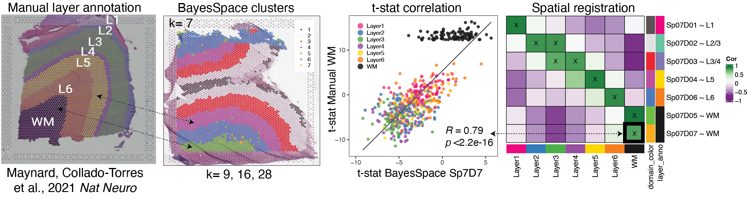
The spatial annotation process correlates the $t$-statistics from the gene enrichment analysis between spatial features from the reference data set, with the $t$-statistics from the gene enrichment of features in the query data set. Pairs with high positive correlation show where similar patterns of gene expression are occurring and what anatomical feature the new spatial feature or cell population may map to.

Overview of the Spatial Registration method

1. Perform gene set enrichment analysis between spatial features (ex. anatomical features, histological layers) on reference spatial data set. Or access existing statistics.

2. Perform gene set enrichment analysis between features (ex. new annotations, data-driven clusters) on new query data set.

3. Correlate the $t$-statistics between the reference and query features.

4. Annotate new spatial features with the most strongly associated reference feature.

5. Plot correlation heat map to observe patterns between the two data sets.

{width=100%}

How to run Spatial Registration with spatialLIBD tools

Introduction.

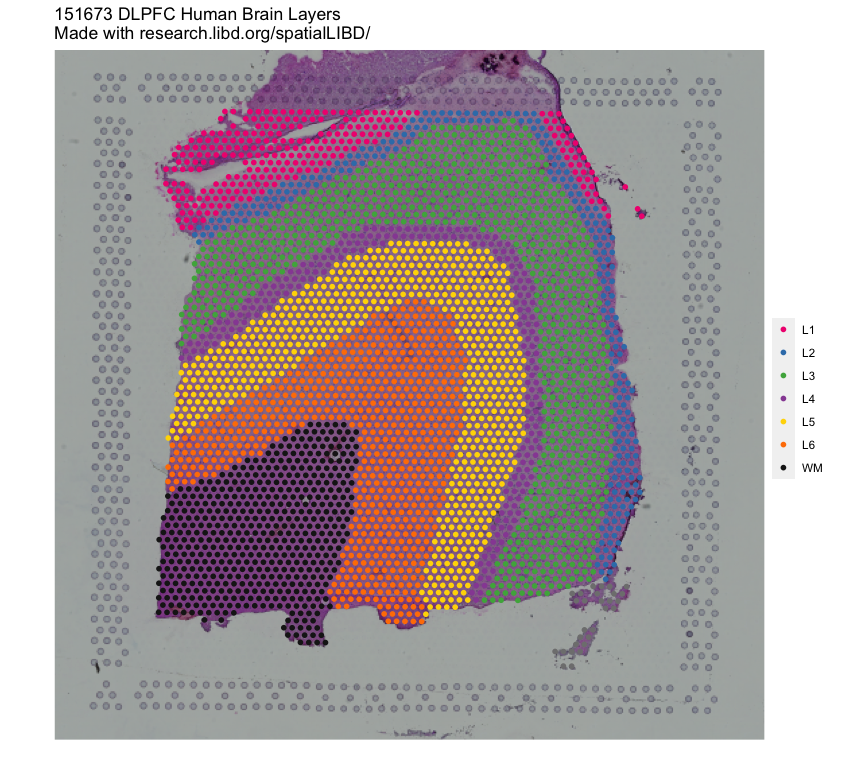
In this example we will utilize the human DLPFC 10x Genomics Visium dataset from Maynard, Collado-Torres et al. r Citep(bib[['spatialLIBDpaper']]) as the reference. This data contains manually annotated features: the six cortical layers + white matter present in the DLPFC. We will use the pre-calculated enrichment statistics for the layers, which are available from r Biocpkg("spatialLIBD").

{width=100%}

The query dataset will be the DLPFC single nucleus RNA-seq (snRNA-seq) data from r Citep(bib[['tran2021']]).

We will compare the gene expression in the cell type populations of the query dataset to the annotated layers in the reference.

Important Notes

Required knowledge

It may be helpful to review Introduction to spatialLIBD vignette available through GitHub or Bioconductor for more information about this data set and R package.

Citing spatialLIBD

We hope that r Biocpkg("spatialLIBD") will be useful for your research. Please use the following information to cite the package and the overall approach. Thank you!

## Citation info
citation("spatialLIBD")

Setup

Install spatialLIBD

if (!requireNamespace("BiocManager", quietly = TRUE)) {
    install.packages("BiocManager")
}

BiocManager::install("spatialLIBD")

## Check that you have a valid Bioconductor installation
BiocManager::valid()

Load required packages

library("spatialLIBD")
library("SingleCellExperiment")

Download Data

Spatial Reference

The reference data is easily accessed through r Biocpkg("spatialLIBD"). The modeling results for the annotated layers is already calculated and can be accessed with the fetch_data() function.

This data contains the results form three models (anova, enrichment, and pairwise), we will use the enrichment results for spatial registration. The tables contain the $t$-statistics, p-values, and gene ensembl ID and symbol.

## get reference layer enrichment statistics
layer_modeling_results <- fetch_data(type = "modeling_results")

layer_modeling_results$enrichment[1:5, 1:5]

Query Data: snRNA-seq

For the query data set, we will use the public single nucleus RNA-seq (snRNA-seq) data from r Citep(bib[['tran2021']]) can be accessed on github.

This data is also from postmortem human brain DLPFC, and contains gene expression data for 11k nuclei and 19 cell types.

We will use BiocFileCache() to cache this data. It is stored as a SingleCellExperiment object named sce.dlpfc.tran, and takes 1.01 GB of RAM memory to load.

# Download and save a local cache of the data available at:
# https://github.com/LieberInstitute/10xPilot_snRNAseq-human#processed-data
bfc <- BiocFileCache::BiocFileCache()
url <- paste0(
    "https://libd-snrnaseq-pilot.s3.us-east-2.amazonaws.com/",
    "SCE_DLPFC-n3_tran-etal.rda"
)
local_data <- BiocFileCache::bfcrpath(url, x = bfc)

load(local_data, verbose = TRUE)

DLPFC tissue consists of many cell types, some are quite rare and will not have enough data to complete the analysis

table(sce.dlpfc.tran$cellType)

The data will be pseudo-bulked over donor x cellType, it is recommended to drop groups with < 10 nuclei (this is done automatically in the pseudobulk step).

table(sce.dlpfc.tran$donor, sce.dlpfc.tran$cellType)

Get Enrichment statistics for snRNA-seq data

spatialLIBD contains many functions to compute modeling_results for the query sc/snRNA-seq or spatial data.

The process includes the following steps

1. registration_pseudobulk(): Pseudo-bulks data, filter low expressed genes, and normalize counts
2. registration_mod(): Defines the statistical model that will be used for computing the block correlation
3. registration_block_cor() : Computes the block correlation using the sample ID as the blocking factor, used as correlation in eBayes call
4. registration_stats_enrichment() : Computes the gene enrichment $t$-statistics (one group vs. All other groups)

The function registration_wrapper() makes life easy by wrapping these functions together in to one step!

## Perform the spatial registration
sce_modeling_results <- registration_wrapper(
    sce = sce.dlpfc.tran,
    var_registration = "cellType",
    var_sample_id = "donor",
    gene_ensembl = "gene_id",
    gene_name = "gene_name"
)

Extract Enrichment t-statistics

## extract t-statics and rename
registration_t_stats <- sce_modeling_results$enrichment[, grep("^t_stat", colnames(sce_modeling_results$enrichment))]
colnames(registration_t_stats) <- gsub("^t_stat_", "", colnames(registration_t_stats))

## cell types x gene
dim(registration_t_stats)

## check out table
registration_t_stats[1:5, 1:5]

Correlate statsics with Layer Reference

cor_layer <- layer_stat_cor(
    stats = registration_t_stats,
    modeling_results = layer_modeling_results,
    model_type = "enrichment",
    top_n = 100
)

cor_layer

Explore Results

Now we can use these correlation values to learn about the cell types.

Create Heatmap of Correlations

We can see from this heatmap what layers the different cell types are associated with.

• Oligo with WM

• Astro with Layer 1

• Excitatory neurons to different layers of the cortex

• Weak associate with Inhibitory Neurons

layer_stat_cor_plot(cor_layer, max = max(cor_layer))

Annotate Cell Types by Top Correlation

We can use annotate_registered_clusters to create annotation labels for the cell types based on the correlation values.

anno <- annotate_registered_clusters(
    cor_stats_layer = cor_layer,
    confidence_threshold = 0.25,
    cutoff_merge_ratio = 0.25
)

anno

Reproducibility

The r Biocpkg("spatialLIBD") package r Citep(bib[["spatialLIBD"]]) was made possible thanks to:

• R r Citep(bib[["R"]])
• r Biocpkg("BiocStyle") r Citep(bib[["BiocStyle"]])
• r CRANpkg("knitr") r Citep(bib[["knitr"]])
• r CRANpkg("RefManageR") r Citep(bib[["RefManageR"]])
• r CRANpkg("rmarkdown") r Citep(bib[["rmarkdown"]])
• r CRANpkg("sessioninfo") r Citep(bib[["sessioninfo"]])
• r CRANpkg("testthat") r Citep(bib[["testthat"]])

This package was developed using r BiocStyle::Biocpkg("biocthis").

Code for creating the vignette

## Create the vignette
library("rmarkdown")
system.time(render("guide_to_spatial_registration.Rmd", "BiocStyle::html_document"))

## Extract the R code
library("knitr")
knit("guide_to_spatial_registration.Rmd", tangle = TRUE)

Date the vignette was generated.

## Date the vignette was generated
Sys.time()

Wallclock time spent generating the vignette.

## Processing time in seconds
totalTime <- diff(c(startTime, Sys.time()))
round(totalTime, digits = 3)

R session information.

## Session info
library("sessioninfo")
options(width = 120)
session_info()

Bibliography

This vignette was generated using r Biocpkg("BiocStyle") r Citep(bib[["BiocStyle"]]) with r CRANpkg("knitr") r Citep(bib[["knitr"]]) and r CRANpkg("rmarkdown") r Citep(bib[["rmarkdown"]]) running behind the scenes.

Citations made with r CRANpkg("RefManageR") r Citep(bib[["RefManageR"]]).

## Print bibliography
PrintBibliography(bib, .opts = list(hyperlink = "to.doc", style = "html"))

LieberInstitute/spatialLIBD documentation built on May 12, 2024, 12:22 a.m.