In jcduda/td2pLL: Fitting a time-dose two-parameter log-logistic model to time-dose-response data

---

title: Time-Dose Two-parameter Log-Logistic Model (td2pLL) output: github_document: pandoc_args: --webtex

---

knitr::opts_chunk$set(
  collapse = TRUE,
  comment = "#>",
  fig.path = "man/figures/README-",
  out.width = "100%"
)
# library(knitr)
# library(td2pLL)

The goal of td2pLL is to fit and display time-dose two-parameter log-logistic (td2pLL) models to appropriate data, e.g. cytotoxicity data and to calculate D-optimal designs for experimental planning. The td2pLL model is defined as

[ f(t, d) = 100-100\frac{d^h}{ED_{50}(t)^h + d^h} ]

with

[ ED_{50} =\Delta \cdot t^{-\gamma} + C_0 . ]

Installation

``` {r, eval = FALSE}

install.packages("devtools")

devtools::install_github("jcduda/td2pLL", build_vignettes = TRUE)

## Example 1: Plot a td2pLL model fit


```r
library(td2pLL)
library(dplyr)
data(cytotox)
# Use subset of compound ASP
data_subset <- cytotox[cytotox$compound == "ASP", c("expo", "dose", "resp")]
colnames(data_subset)[1] <- "time"
fit <- fit_td2pLL(data = data_subset)
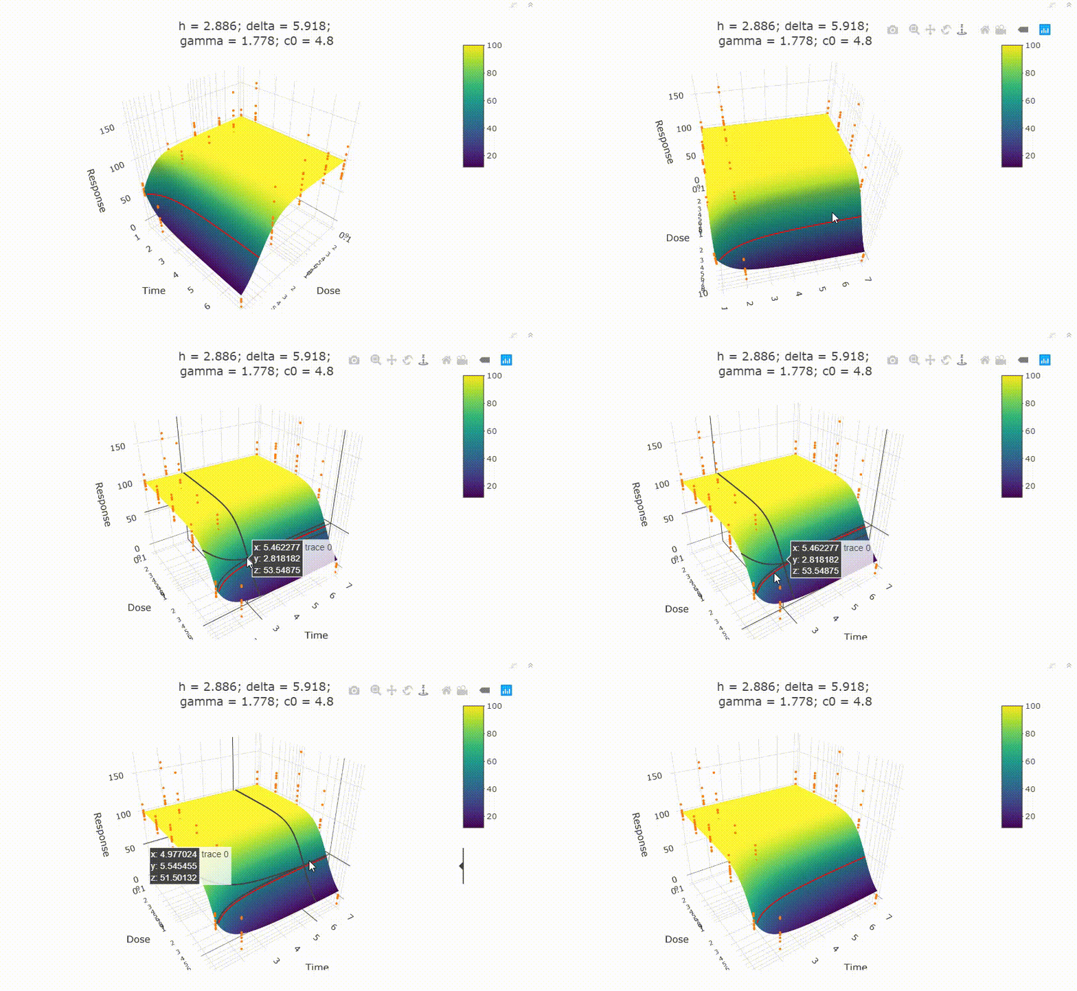
# In your Viewer in R Studio, you will see this when uncommenting the following line
# plot(fit)

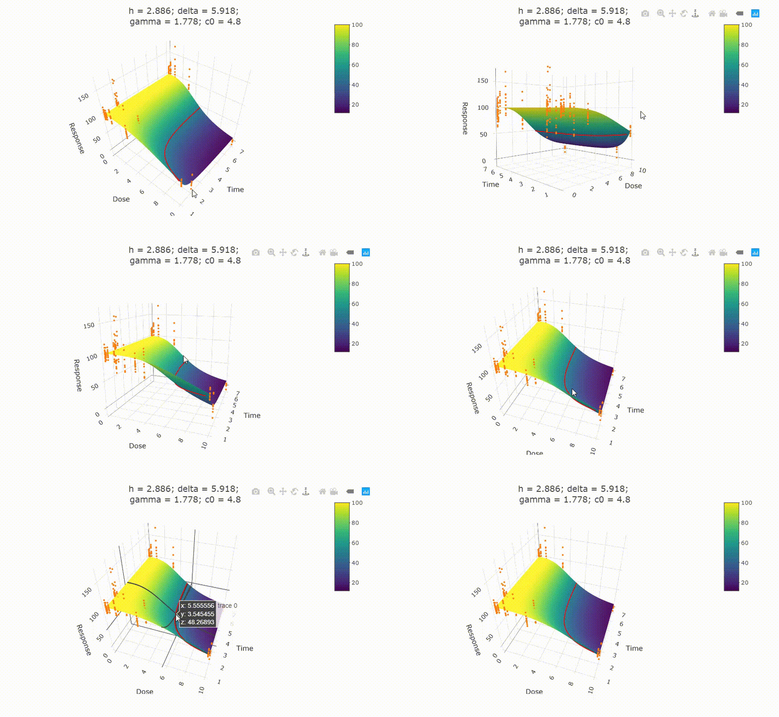
# change scale of dose axis to linear scale, so that dose=0 can be displayed: 
# plot(fit, xaxis_scale = "linear")
# uncommenting the above line will show you the following in the Viewer or R Studio

# Details on fit:
summary(fit)
# Calculate ED50 values at different (exposure) times:
get_ED50s(coefs = coef(fit), times = c(1, 2, 3))

Example 2: Use two-step pipeline for conditional time-dose modeling

If you are not sure if you need to model time-dependency, you can use the two-step anova-based pipeline using TDR(). In an initial step, via nested anova it is checked if the time has an influence. Specifically, a 2pLL model with upper and lower limit set to 100 and 0, respectively, that ignores the epxosure time component is the null model. The full model is a 2pLL model where for each exposure time, a different $ED_{50}$ parameter is fitted. Only the $h$ parameter is shared across exposure times. If the anova test between these nested models is significant, an effect of the exposure time is assumed to be true. In thas case, a td2pLL model is fitted in the second step, the modeling step. If the pre-test does not yield a significant result, then the regualr 2pLL model with upper and lower limit 100 and 0, respectively, is fitted.

For the data of the above chosen compound, ASP, an influence of the exposure time on the viability was detected.

TDR_res <- TDR(data = data_subset)
TDR_res
# Uncomment to see in Viewer
#plot(TDR_res$fit)

If we instead look at the measurements for the BOS compound and reduce the data set a bit to a more realistic size, the pre-test suggests to NOT model the time-dependency. Therefore, only a one-dimensionl 2pLL model is fitted.

Note that if the data set is large enough, the anova pre-test will always propose to model the time-effect as it will always find a significant (but possibly irrelevant) difference in $ED_{50}$ values between exposure periods.

This significance-vs-relevance problem is always present in classical frequentist statistical hypothesis testing.

data_subset <- cytotox[cytotox$compound == "BOS" &
                         cytotox$dose %in% c(0, 0.1, 0.316, 1),
                       c("expo", "dose", "resp")]
data_subset <- data_subset %>% group_by(expo, dose) %>%
  dplyr::filter(dplyr::row_number() <= 3)
colnames(data_subset)[1] <- "time"
TDR_res <- TDR(data = data_subset)
TDR_res$pretest
plot(TDR_res$fit, type = "all")

Example 3: D-optimal design

Optimal design theory is highly developed and also well established in pharmaceutical dose-finding studies.

For a D-optimal design of a td2pLL models, we no longer assume the response-mean at control to be known( $E_0$=100). This has the effect that the optimal design proposes to have experiments at the control (dose=0), which cannot be dismissed in practical application.

One can choose, however if the response-level for infitiely large doses should be assumed to be known (e.g. $Emax = -100$ for response=0 for large doses).

If it is assumed to be known, the resulting optimal design will not propose to measure at these high doses, as the response is assumed known there and measurements at these high doses would not help to gain further knowledge about the dose-time-response relationship.

The numerical back-bone is the Imperialist Competitive Algorithm (ICA) by Masoudi et al. (2017).

It will take a few minutes to be calculated. Change to plot_cost=TRUE to follow the optimization process.

td_opt_1 <- td_opt(param = c(h = 2, delta = 0.2, gamma = 1.3, c0 = 0.2),
                   Emax_known = TRUE, 
                   # lower limit for time and dose
                   lx = c(1, exp(-8)),
                   # upper limit for time and dose
                   ux = c(10, 1),
                   # Choose trace=TRUE to follow the optimization process
                   ICA.control = list(ncount = 200, rseed = 1905, trace = FALSE,
                                      plot_cost = FALSE),
                   iter = 400)
td_opt_1

The final design contains 7 time-dose points, where one will be placed at the smallest dose-value with weight 0.2. The smallest dose-level can be interpreted as dose=0.

If desired, this point can be splitted along the time-axis. This means that instead of having 20 \% of observations at dose = 0 and time = 6.2, one can euivalently choose

• 20/3 \% at dose = 0 and time = 1
• 20/3 \% at dose = 0 and time = 10 and
• 20/3 \% at dose = 0 and time = 2.2.

plot_td_des(td_opt_1)

One can check if the design is indeed optimal with a sensitivity plot. If the entire plot is approximately below 0 at all points in the design space and approximately zero at the proposed design points, then the design is D-optimal for the assumed paramter.

plot_td_dcrit_equ(td_opt_1, 
                  # to rotate the plot
                  plot_phi = 30)

jcduda/td2pLL documentation built on May 14, 2022, 6:48 p.m.