README.md
In qwang-big/irene: R interface to interactive epigenetic analysis
Irene: Integrative Ranking with Epigenetic Network of Enhancers

Irene is an R package which allows you
- Find significantly altered genes between two biological conditions from histone ChIP-Seq and DNA methylation tracks (BigWig)
- Focus on the genes which are associated with more extensive epigenetic modification over targetting enhancers.
- Annotate and visualize the global epigenetic variances with network analysis.
Using Irene, we analyzed the epigenetic networks from multiple histone marks and DNA methylation in Roadmap, BLUEPRINT, and CEEHRC, and the results are presented in http://hdsu-bioquant.github.io/irene-web/.
INTRODUCTION
Irene is developed for two purposes in epigenetic ranking:
- Integrate several epigenetic marks
- Incorporate enhancers
With the help of Irene, user not only discover the genes which show significantly epigenetic alterations on their promoters, but also the ones which are connected with strong epigenetic modifications on neighbouring enhancers, which are presented as increased/decreased rankings (Fig. 1)
 Fig. 1 Genes with more enhancer alterations have higher rank
The whole idea has been demonstrated in the Chapter III of Qi Wang's dissertation. For the above purposes, we employed singular value decomposition dPCA and random walk ranking PageRank. The epigenetic alterations over genomic regulatory elements between two groups are presented as dPC scores and further to PageRank scores during solving the enhancer-promoter relationships.
Installation
Irene can be installed directly from GitHub with the help of devtools package:
library(devtools)
install_github("hdsu-bioquant/irene")
If you have problems in intalling the package, please have a look at FAQs.
For impatient people
If you do not have the various datasets needed in the following sections, please follow the supplymentary, where we have prepared all the necessary input needed for performing the tests. In the test cases, you can understand the data structures, procedures, and the outputs of Irene.
Prerequisites
Genomic regions to be tested
User need to provide promoter and enhancer regions to compare their differential epigenetic modifications. We also provide pre-defined promoters from The Eukaryotic Promoter Database and pre-defined from GeneHancer.
Given that the enhancers from GeneHancer database are an ensemble of all tissues/cell types, one may need to filter out the unspecific ones, which can be done by overlapping with the enhancer-specific histone marks, e.g., histone H3 lysine 4 monomethylation (H3K4me1) or the histone 3 lysine 27 acetylation (H3K27ac) marks.
Promoter-enhancer (P-E) interactions
Enhancers within 1Mb distance to the transcription start site (TSS) are considered potential promoter-interacting ones. In a common sense, the interactions should not cross the topologically associating domains (TAD) boundary. Therefore, we compiled a cell-type specific enhancer-promoter interaction list by excluding the interactions outside the same TAD from GSE87112. Enhancer-promoter interactions probability are estimated using a power-law decay function based on the distances to the TSS. Enhancer-promoter distances for sample tissues can be downloaded from https://github.com/hdsu-bioquant/irene-data/PEdistances, including:
- H1: H1 human embryonic stem cell line
- MES: H1 BMP4 derived mesendoderm cultured cells
- MSC: H1 derived mesenchymal stem cells
- NPC: H1 derived neural precursor cells
- TPC: H1 derived trophoblast stem cells
In practice, as TADs between different cell types are relative conserved (Schmitt AD, 2016), one can use the H1 cell line in case the TAD of corresponding cell type is not available.
Epigenetic intensity data
Irene requires user to provide BigWig format to represent the sequencing density of BS-Seq or ChIP-Seq. To begin with, user need to create a data.frame named meta indicating the location of the BigWig files, as well as groups and experiment types (as dataset column).
Here is a sample as follows (click to uncollapse):
| | file | group | dataset |
|----|------------------------------------------------------------------------------------|-------|---------|
| 1 | UCSD.H1_Derived_Mesenchymal_Stem_Cells.Bisulfite-Seq.methylC-seq_h1-msc_r1a.wig.bw | 1 | 1 |
| 2 | UCSD.H1_Derived_Mesenchymal_Stem_Cells.Bisulfite-Seq.methylC-seq_h1-msc_r2a.wig.bw | 1 | 1 |
| 3 | UCSD.H1_Derived_Mesenchymal_Stem_Cells.H3K27ac.SK436.wig.bw | 1 | 2 |
| 4 | UCSD.H1_Derived_Mesenchymal_Stem_Cells.H3K27ac.SK438.wig.bw | 1 | 2 |
| 5 | UCSD.H1_Derived_Mesenchymal_Stem_Cells.H3K27me3.SK437.wig.bw | 1 | 3 |
| 6 | UCSD.H1_Derived_Mesenchymal_Stem_Cells.H3K27me3.SK439.wig.bw | 1 | 3 |
| 7 | UCSD.H1_Derived_Mesenchymal_Stem_Cells.H3K9ac.SK518.wig.bw | 1 | 4 |
| 8 | UCSD.H1_Derived_Mesenchymal_Stem_Cells.H3K9ac.SK519.wig.bw | 1 | 4 |
| 9 | UCSD.H1_Derived_Mesenchymal_Stem_Cells.H3K9me3.SK507.wig.bw | 1 | 5 |
| 10 | UCSD.H1_Derived_Mesenchymal_Stem_Cells.H3K9me3.SK508.wig.bw | 1 | 5 |
| 11 | UCSD.H1_Derived_Mesenchymal_Stem_Cells.Input.SK443.wig.bw | 1 | 6 |
| 12 | UCSD.H1_Derived_Mesenchymal_Stem_Cells.Input.SK444.wig.bw | 1 | 6 |
| 13 | GSM429321_UCSD.H1.Bisulfite-Seq.methylC-seq_h1_r2a.bw | 2 | 1 |
| 14 | GSM429322_UCSD.H1.Bisulfite-Seq.methylC-seq_h1_r2b.bw | 2 | 1 |
| 15 | GSM432685_UCSD.H1.Bisulfite-Seq.methylC-seq_h1_r1a.bw | 2 | 1 |
| 16 | GSM432686_UCSD.H1.Bisulfite-Seq.methylC-seq_h1_r1b.bw | 2 | 1 |
| 17 | UCSD.H1.H3K27ac.LL313.bw | 2 | 2 |
| 18 | UCSD.H1.H3K27ac.SAK270.bw | 2 | 2 |
| 19 | UCSD.H1.H3K27me3.LL241.bw | 2 | 3 |
| 20 | UCSD.H1.H3K27me3.LL314.bw | 2 | 3 |
| 21 | UCSD.H1.H3K27me3.YL95.bw | 2 | 3 |
| 22 | UCSD.H1.H3K9ac.LL240.wig.bw | 2 | 4 |
| 23 | UCSD.H1.H3K9ac.SAK68.wig.bw | 2 | 4 |
| 24 | UCSD.H1.H3K9me3.AK54.wig.bw | 2 | 5 |
| 25 | UCSD.H1.H3K9me3.LL218.wig.bw | 2 | 5 |
| 26 | UCSD.H1.H3K9me3.YL75.wig.bw | 2 | 5 |
| 27 | UCSD.H1.H3K9me3.YL77.wig.bw | 2 | 5 |
| 28 | UCSD.H1.Input.AK57.wig.bw | 2 | 6 |
| 29 | UCSD.H1.Input.DM219.wig.bw | 2 | 6 |
| 30 | UCSD.H1.Input.LL-H1-I1.wig.bw | 2 | 6 |
| 31 | UCSD.H1.Input.LL-H1-I2.wig.bw | 2 | 6 |
| 32 | UCSD.H1.Input.LLH1U.wig.bw | 2 | 6 |
| 33 | UCSD.H1.Input.YL154.wig.bw | 2 | 6 |
| 34 | UCSD.H1.Input.YL208.wig.bw | 2 | 6 |
| 35 | UCSD.H1.Input.YL262.wig.bw | 2 | 6 |
| 36 | UCSD.H1.Input.YL328.wig.bw | 2 | 6 |
The BigWig files for our test cases were converted from wig files retrieved from NIH Roadmap Epigenomics Project data gateway, BLUEPRINT, and CEEHRC, respectively. Precompiled R objects in our test cases can be retrieved from here
USAGE
R environment for the test cases.
The following options were set up during performing our tests.
options(stringsAsFactors = FALSE)
Load pre-defined regions
The pre-defined promoter and enhancer regions with corresponding IDs (precompiled hg19, hg38) need to be loaded first with:
bed <- read.table('https://raw.githubusercontent.com/hdsu-bioquant/irene-data/master/promenh.hg19.bed')
Import sequencing density data from BigWig files
The datasets are prepared from BigWig files by users. User needs to create a data.frame named meta first using the BigWig files under current working directory, and Irene uses the bigWigAverageOverBed program as follows, which can process BigWig files with multi-threads.
data <- importBW(meta, bed)
Alternatively, users can prepare the same R data objects with cluster computing, following the sample procedure by themselves. Irene reads the data from bigWigAverageOverBed outputs into another data.frame named data over the input genomic regions. Afterwards, user needs to edit meta manually, which must contain file, group, dataset information (a sample meta is here)
Filter out unspecific enhancers
We only took the regions which are more likely to be true enhancers, therefore the following function is used to get the indices which overlapped with enhancer histone marks (H3K4me1 in the following case). The peaks identified by Roadmap Epigenetics Project were retrieved from http://egg2.wustl.edu/roadmap/data/byFileType/peaks/consolidated, and run:
i <- filterPeak(c("GSM3444631.bed","GSM3444640.bed","GSM3444652.bed","GSM3444655.bed",
    "GSM3444653.bed","GSM3444654.bed","GSM3444656.bed"), bed, group=c(1,1,1,1,2,2,2))
| Cancer / primary cells | Controls |
|------------------------|----------|
| Chronic Lymphocytic Leukemia (CLL) | Naive B Cell |
| Acute Lymphoblastic Leukaemia (ALL) | Naive B Cell |
| Acute Myeloid Leukaemia (AML) | Naive B Cell |
| Multiple Myeloma (MM) | Naive B Cell |
| Mantle Cell Lymphoma (MCL) | Naive B Cell |
| Chronic Lymphocytic Leukemia (mutated) (mCLL) | Naive B Cell |
| Colorectal Cancer (CRC) | Sigmoid Colon |
| Lower Grade Glioma (LGG) | Normal Brain |
| Papillary Thyroid Cancer (PTC) | Normal Thyroid |
| Mesenchymal Stem Cells (MSC) | Embryonic Stem Cells |
| Neural Progenitor Cells (NPC) | Embryonic Stem Cells |
| Trophoblast Stem Cells (TSC) | Embryonic Stem Cells |
| H1 BMP4 derived Mesendoderm (MES) | Embryonic Stem Cells |
| Glioblastoma (GB) subtype IDH | GB subtype MES |
| Glioblastoma (GB) subtype RTK I | GB subtype MES |
| Glioblastoma (GB) subtype RTK II | GB subtype MES |
Full R code for analyzing the above datasets is in the supplymentary. For the CLL test case, which is already incorporated in the package, one can simply load necessary dataset with:
data(CLL)
Measure combinatorial effect of epigenetic alterations
We use dPCA(Ji H, 2013) to measure combinatorial effect of epigenetic alterations. The software is already integrated into Irene as an external C function. User can select a subset of datasets to study, for the CLL test case:
j <- c(1,2,6,8)
Use the following command to read the data which were selected with index i:
res <- dPCA(meta, bed[i,], data[i,], datasets=j, transform=j, normlen=j, verbose=TRUE)
or the following if all the genomic regions are to be tested.
res <- dPCA(meta, bed, data, datasets=j, transform=j, normlen=j, verbose=TRUE)
The output res is a named list which has three keys: gr, Dobs, and proj.
- gr
contains the pre-defined regions followed by the computed PCs from dPCA. A sample output may look like this:
| seqnames | start | end | id | PC1 | PC2 | PC3 |
|----------|-----------|-----------|------------|----------|------------|------------|
| chr5 | 159099769 | 159099829 | EBF1_1 | 22.12935 | -11.913720 | -1.9786781 |
| chr19 | 53869401 | 53869461 | MYADM_3 | 22.12694 | -8.876568 | 3.7468742 |
| chr4 | 52862267 | 52862327 | RASL11B_1 | 21.89510 | -14.516893 | -4.8862062 |
| chr8 | 141099562 | 141099711 | GH08I141099 | 21.88550 | 7.578159 | 1.3920079 |
| chr6 | 131063357 | 131063417 | EPB41L2_4 | 21.57229 | -12.886749 | -0.8408109 |
| chr2 | 158457054 | 158457114 | PKP4_1 | 21.42755 | -8.421447 | -4.6387676 |
The table is sorted descendingly by PC1
-
Dobs
The D matrix, which contains the observed differences between the two conditions. This is the data analyzed by dPCA.
-
proj
Estimated beta coefficients for each dPC.
The contribution of each histone mark to the PCs can be visualized with the following function:
plotD(res$Dobs, c("K4me1", "K4me3", "K27ac", "Meth"), scales::percent(res$proj['percent_var',]))
Infer promoter-enhancer interaction probabilities according to distances
Use the following function to convert the promoter-enhancer interactions in a given range of TSS (1Mb in the data provided) to probabilities of interaction.
- We first load the P-E interactions in H1ESC cell line, the three columns in H1 data.frame are enhancer IDs, promoter IDs, P-E distances, respectively.
H1 <- read.table('https://raw.githubusercontent.com/hdsu-bioquant/irene-data/master/PEdistances/H1.hg19.pair')
- Then transform the P-E interactions from bp to Mb:
H1[,3] <- abs(H1[,3]/1e6)
- We apply a power-decay function to represent the likelihood of P-E interactions. The power-coefficient is estimated from several capture Hi-C datasets Mifsud et al, 2015, Javierre et al, 2016, Rubin et al, 2017, which is explained in Figure 3.11 and Figure 3.14b of Qi Wang's dissertation. We recommand using -20 for all the test cases.
H1[,3] <- exp(-20*H1[,3]+1)
Using PageRank to rank the epigenetic alterations from both enhancers and promoters.
The PageRank function will take in the alteration contribution from enhancers, resulting in higher ranks of associated promoters if targeted by highly altered enhancers.
res$pg <- pageRank(res$gr, H1)
, where res$pg contains rankings generated from PC1 to PCn. If one is interested in the second PC, it can be accessed by:
res$pg$PC2
Get the rank of only promoters as well, which will be used to compare with the PageRank rankings.
Use the following function to get the rank of the promoters according to PC1. A higher rank indicates stronger alterations of the corresponding gene.
res$pg$prom <- getPromId(res$gr, pc="PC1")
Use literature-derived marker genes as a metric for evaluating the ranking
Cancer and cell-type specific marker genes are listed in Table S2 & 3 of Qi Wang's disseration, which are already compiled as an R object and can be loaded with:
data(markers)
The Empirical Cumulative Distribution Function (ECDF) of the marker gene positions in each ranking list can be plotted with:
plotRank(res$pg, markers$CLL)
, where the CLL marker genes for this test are ordered according to the positions of their rankings (Fig. 2), and the area under the curve (AUC) of each ranking list is described in the legend.
Fig. 2 CLL marker gene positions along the ROC curves
Network analysis of the enriched pathways of significantly epigeneticaly alterated genes
Network analysis groups highly-ranked genes according to known gene interaction databases, and further searches clusters of genes in biological function databases. In this case, we loaded Human Protein Reference Database (HPRD) for grouping genes:
data(hprd)
, and set the edge weights in accordance with the average rank of the two connected genes, which is done by:
g <- edgeRank(res$pg$PC1, hprd)
, where we created a weighted HPRD networks using the edge weights calculated from the PC1 of the genes.
Using random walk clustering, we got a list of top-ranked sub-networks with desired number, e.g., 15 sub-networks:
res$gs <- exportMultinets(g, 15)
, and the sub-networks were searched in WikiPathways and KEGG for enrichment of biological functions:
res$ga <- annotNets(res$gs)
Outputs
The following commands need to be executed to generate HTML outputs for interactive exploration of the enriched networks, epigenetic tracks, rank comparisons and benchmarking (ROC curves).
To begin with, a prefix variable should be set corresponding to the experiment first, as for this test case we set:
prefix = "CLL"
The files are created in the current working directory if not mentioned explicitly. Use the following commands to create a specific folder for the outputs (e.g., a sub-directory in the home folder):
dir.create("~/CLLoutput")
setwd("~/CLLoutput")
Write the two ranking list to a CSV file for comparison, significance of the genes from the highest to the lowest are ordered from the top to the bottom of the list.
writeRank(res$pg[[1]], res$pg$prom, prefix)
Write the normalized epigenome signals of the two groups, labels of the two groups are provided by user.
writeData(res$gr, c("CLL", "Bcell"), prefix)
Export the principal components of epigenetic marks
exportD(res$Dobs, c('K4me1','K4me3','K27ac','Meth'), "CLL")
, and the sub-networks list was saved to a JSON with each network structure:
exportJSONnets(res$gs, prefix)
In addition, the enriched pathways of the sub-networks are also saved as JSON file:
exportJSONpathways(res$ga, prefix, n=15)
Export the meta info to a CSV file if you have not done that before.
write.csv(meta,paste0(prefix,"meta.csv"))
Finally, create an index page in the same directory with above JSON files for visualizing in an internet browser:
exportApps(prefix, markers['CLL'])
Interpreting the results
The above mentioned test cases are hosted in another repository http://hdsu-bioquant.github.io/irene-web, in which the outputs are presented in the following four sections:
Rank list
For every test case, Irene produced two rank lists: one is from PageRank score (generated from promoter and enhancer scores, as well as P-E interactions, therefore abbreviated as PromEnh), another is from the PC1 scores of promoters (abbreviated as PromOnly). Both lists are contained in a CSV file for downloading, which looks like:
| | PromEnh | PromOnly |
|--|--------|----------|
| 1| MED13L | CBWD5 |
| 2| CBLB | CBWD3 |
| 3| VAV3 | CBWD7 |
| 4| LPP | SERF1B |
| 5| NOTCH2 | SERF1A |
| 6| MKLN1 | HIST2H4A |
| 7| ARHGAP15 | HIST2H4B |
| 8| BACH2 | GTF2H2 |
| 9| MGAT5 | NOTCH4 |
...
, where the genes are ordered from the most significant to the least significant in both lists, and the line numbers correspond to the positions in the lists.
Plotting the positions of each gene in a two-dimensional graph allows one to inspect the level of significance regarding the promoters or enhancers of a gene, whereas the genes under high enhancer/low promoter regulation are placed at the bottom-right corner of the graph. In the above CLL test case, the result implies many genes are ranked higher considering the enhancer alterations. The baseline became distorted for those genes who did not receive contribution from enhancers.
During benchmarking, The selected marker genes, as well as genes from other collections (COSMIC, MalaCards, IntOGen) are listed besides the graph, so that the genes are highlighted in red upon clicking the corresponding item. Additional information are shown as mouse-over tooltips or links in the pop-ups.
 Fig. 3 Exploring ranking plot interface (user guide)
Network enrichment
In these network presentations, the enriched sub-networks are ordered based on the average significance of the their nodes, wherein the left-side of the node represents its rank in the PromEnh list, and the right-side of the node represents its rank in the PromOnly list. Pathways of each sub-network are tested with EnrichR, and the ones which are significantly enriched in KEGG and WikiPathways are listed. Upon clicking an item in the drop list of pathways, the corresponding genes in that pathway are highlighted in red. Additional information are shown as mouse-over tooltips or links in the pop-ups.
Fig. 4 Exploring network browser interface (user guide)
Epigenome heatmap
The epigenome heatmap serves as an interactive browser of normalized epigenetic signals, wherein tracks from different samples are aligned in accordance with biological conditions and epigenetic marks. In this presentation, the whole genome is divided into bins with fixed length (2kb in this test case). To preserve storage space, only the bins overlaped with the provided promoter/enhancer regions are rendered, leaving the rest of the genome in background color. The topmost track represent the regulatory genomic elements (promoters/enhancers), and the colors in this track correspond to their PC1 scores. Furthermore, the promoter of the gene name is centered upon user's input. The triangles above the regulatory elements represent the referred targets from the available resources in the drop list (GeneHancer interactions by default). The other tracks represent the data intensities, wherein the colors correspond to the normalized epigenetic signals. Additional information are shown as mouse-over tooltips or links in the pop-ups.
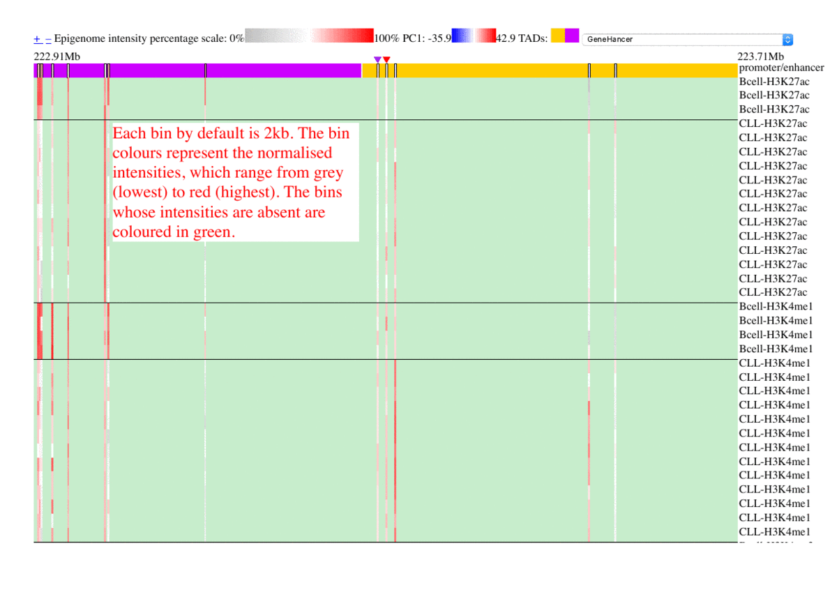 Fig. 5 Exploring epigenome browser interface (user guide)
Hallmark ROC
The receiver operating characteristic (ROC) curves represent the ECDF of marker genes (curated for benchmarking, COSMIC, MalaCards, IntOGen) of the two rank lists (PromEnh and PromOnly). The curves are updated upon clicking the item listed besides the graph.
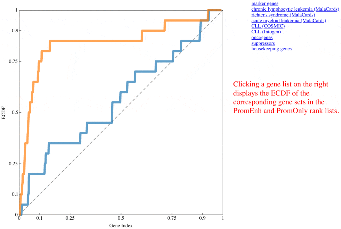
Fig. 6 Exploring ROC plot interface (user guide)
Case studies
Epigenetic and expression data were downloaded from EdaccData Release-9, CEEHRC, BLUEPRINT.
Acknowledgements
The results presented here are in part based upon data generated by The Canadian Epigenetics, Epigenomics, Environment and Health Research Consortium (CEEHRC) initiative funded by the Canadian Institutes of Health Research (CIHR), Genome BC, and Genome Quebec. Information about CEEHRC and the participating investigators and institutions can be found at http://www.cihr-irsc.gc.ca/e/43734.html.
References
- Schmitt AD, Hu M, Jung I, et al. A Compendium of Chromatin Contact Maps Reveals Spatially Active Regions in the Human Genome. Cell Reports. 2016;17(8):2042–2059.
- Ji H, Li X, Wang Qf, et al. Differential principal component analysis of ChIP-seq. Proceedings of the National Academy of Sciences. 2013;110(17):6789–6794.
FAQs
- Q: Package 'XXX' is not available (for R version 3.x.x).
A: Please install them manually, using:
source("https://bioconductor.org/biocLite.R")
biocLite("GenomeInfoDb","GenomicRanges","IRanges","preprocessCore","S4Vectors","XVector")
For R (version "3.5") and later, please enter:
if (!requireNamespace("BiocManager", quietly = TRUE))
    install.packages("BiocManager")
BiocManager::install(c("preprocessCore","GenomicRanges"), version = "3.8")
- Q: Which operation system is Irene able to run on?
A: We have tested Irene under Linux and Mac OSX. For Microsoft Windows, users need to resolve the compiling library themselves, using such as Cygwin or other C libraries.
- Q: How do I open the website for visualizing the outputs?
A: You can run "run.sh" after exportApps. If it does not work, please run it manually in the console, or use the following command:
python -m SimpleHTTPServer
or
python3 -m http.server
, then navigate to http://localhost:8000/ in your internet browser to see the results.
License
MIT
Supplymentary Info
#download genomic coordinates of promoter and enhancers for reading
URL <- "https://raw.githubusercontent.com/hdsu-bioquant/irene-data/master/promenh.hg19.bed"
BED <- "promenh.hg19.bed"
FUN <- "bigWigAverageOverBed" #or "./bigWigAverageOverBed" if the program is in current folder
download.file(URL, BED)
meta <- data.frame(file=dir('.','*.bigWig$'),group=1,dataset=1,stringsAsFactors=FALSE)
bed  <- read.table(BED,stringsAsFactors=FALSE)
lapply(meta$file,function(f) system(paste0(FUN,' ',f,' ',BED,' ',f,'.out')))
#use mclapply or other batch scripts if you want to start multiple threads, e.g.
#mclapply(meta$file,function(f) system(paste0(FUN,' ',f,' ',BED,' ',f,'.out')), mc.cores = 4)
data <- matrix(unlist(lapply(meta$file,function(f)
    read.table(paste0(f,".out"),stringsAsFactors=FALSE)[,4])), ncol = nrow(meta), byrow = FALSE)
rownames(data) <- read.table(paste0(meta$file[1],".out"),stringsAsFactors=FALSE)[,1]
library(irene)
options(stringsAsFactors = FALSE)
H1=read.table('https://raw.githubusercontent.com/hdsu-bioquant/irene-data/master/PEdistances/H1.hg19.pair')
H1[,3]=abs(H1[,3]/1e6)
H1[,3]=exp(-20*H1[,3]+1)
data(hprd)
data(markers)

case = "NPC"
load(url("https://raw.githubusercontent.com/hdsu-bioquant/irene-data/master/NPC.hg19.rda"))
j = c(1,2,3,5,6)
lbl=c('Meth','K27ac','K27me3','K36me3','K4me1','K4me3','K9ac','K9me3')
data = data[match(bed[,4],rownames(data)),]
npc = dPCA(meta, bed[i,], data[i,], datasets=j, transform=j, normlen=j, verbose=T)
plotD(npc$Dobs, lbl[j], scales::percent(npc$proj['percent_var',]), title=case)
exportD(npc$Dobs, lbl[j], case)
writeData(npc$gr, c("NPC", "ESC"), "NPC")
npc$pg=pageRank(npc$gr, H1, statLog=case, rewire=F)
npc$pg$prom=getPromId(npc$gr)
(npc$auc=plotRank(npc$pg, markers[[case]]))
writeRank(npc$pg[[1]],npc$pg$prom, case)
g=edgeRank(npc$pg[[1]],hprd)
npc$gs=exportMultinets(g, 15, rewire=F)
exportJSONnets(npc$gs, case)
npc$ga = annotNets(npc$gs)
exportJSONpathways(npc$ga, case, n=15)
write.csv(meta,paste0(case,"meta.csv"))
exportApps(case, markers[case])

case = "MSC"
load(url("https://raw.githubusercontent.com/hdsu-bioquant/irene-data/master/MSC.hg19.rda"))
j = c(1,2,3,5,6)
lbl=c('Meth','K27ac','K27me3','K36me3','K4me1','K4me3','K9ac','K9me3')
data = data[match(bed[,4],rownames(data)),]
msc = dPCA(meta, bed[i,], data[i,], datasets=j, transform=j, normlen=j, verbose=T)
plotD(msc$Dobs, lbl[j], scales::percent(msc$proj['percent_var',]), title=case)
exportD(msc$Dobs, lbl[j], case)
writeData(msc$gr, c("MSC", "ESC"), "MSC")
msc$pg=pageRank(msc$gr, H1, statLog=case, rewire=F)
msc$pg$prom=getPromId(msc$gr)
(msc$auc=plotRank(msc$pg, markers[[case]]))
writeRank(msc$pg[[1]],msc$pg$prom, case)
g=edgeRank(msc$pg[[1]],hprd)
msc$gs=exportMultinets(g, 15, rewire=F)
exportJSONnets(msc$gs, case)
msc$ga = annotNets(msc$gs)
exportJSONpathways(msc$ga, case, n=15)
write.csv(meta,paste0(case,"meta.csv"))
exportApps(case, markers[case])

case = "MES"
load(url("https://raw.githubusercontent.com/hdsu-bioquant/irene-data/master/MES.hg19.rda"))
j = c(1,2,3,5,6)
lbl=c('Meth','K27ac','K27me3','K36me3','K4me1','K4me3','K9ac','K9me3')
data = data[match(bed[,4],rownames(data)),]
mes = dPCA(meta, bed[i,], data[i,], datasets=j, transform=j, normlen=j, verbose=T)
plotD(mes$Dobs, lbl[j], title=case)
mes$pg=pageRank(mes$gr, H1, rewire=F)
mes$pg$prom=getPromId(mes$gr)

case = "TSC"
load(url("https://raw.githubusercontent.com/hdsu-bioquant/irene-data/master/TSC.hg19.rda"))
j = c(1,2,3,5,6)
lbl=c('Meth','K27ac','K27me3','K36me3','K4me1','K4me3','K9ac','K9me3')
data = data[match(bed[,4],rownames(data)),]
tsc = dPCA(meta, bed[i,], data[i,], datasets=j, transform=j, normlen=j, verbose=T)
plotD(tsc$Dobs, lbl[j], scales::percent(tsc$proj['percent_var',]), title=case)
exportD(tsc$Dobs, lbl[j], case)
writeData(tsc$gr, c("TSC", "ESC"), "TSC")
tsc$pg=pageRank(tsc$gr, H1, statLog=case, rewire=F)
tsc$pg$prom=getPromId(tsc$gr)
(tsc$auc=plotRank(tsc$pg, markers[[case]]))
writeRank(tsc$pg[[1]],tsc$pg$prom, case)
g=edgeRank(tsc$pg[[1]],hprd)
tsc$gs=exportMultinets(g, 15, rewire=F)
exportJSONnets(tsc$gs, case)
tsc$ga = annotNets(tsc$gs)
exportJSONpathways(tsc$ga, case, n=15)
write.csv(meta,paste0(case,"meta.csv"))
exportApps(case, markers[case])

case = "CLL"
load(url("https://raw.githubusercontent.com/hdsu-bioquant/irene-data/master/CLL.hg19.rda"))
j = c(1,2,6,8)
data = data[match(bed[,4],rownames(data)),]
lbl=c('K4me1','K4me3','K9me3','K27me3','K36me3','K27ac','Input','Meth')
cll = dPCA(meta, bed[i,], data[i,], datasets=j, transform=j, normlen=j, verbose=T)
plotD(cll$Dobs, lbl[j], scales::percent(cll$proj['percent_var',]), title=case)
exportD(cll$Dobs, lbl[j], case)
writeData(cll$gr, c("CLL", "Bcell"), "CLL", intTemp=FALSE)
cll$pg=pageRank(cll$gr, H1, statLog=case, rewire=F)
cll$pg$prom=getPromId(cll$gr)
(cll$auc=plotRank(cll$pg, markers[[case]]))
writeRank(cll$pg[[1]],cll$pg$prom, case)
g=edgeRank(cll$pg[[1]],hprd)
cll$gs=exportMultinets(g, 15, rewire=F)
exportJSONnets(cll$gs, case)
cll$ga = annotNets(cll$gs)
exportJSONpathways(cll$ga, case, n=15)
write.csv(meta,paste0(case,"meta.csv"))
exportApps(case, markers[c(case,"OG")])

case = "PTC"
load(url("https://raw.githubusercontent.com/hdsu-bioquant/irene-data/master/PTC.hg19.rda"))
j = c(1,2,4,6,8)
data = data[match(bed[,4],rownames(data)),]
lbl=c('K4me1','K4me3','K9me3','K27me3','K36me3','K27ac','Input','Meth')
ptc = dPCA(meta, bed[i,], data[i,], datasets=j, transform=j, normlen=j, verbose=T)
plotD(ptc$Dobs, lbl[j], scales::percent(ptc$proj['percent_var',]), title=case)
exportD(ptc$Dobs, lbl[j], case)
writeData(ptc$gr, c("PTC", "Thyroid"), "PTC")
ptc$pg=pageRank(ptc$gr, H1, statLog=case, rewire=F)
ptc$pg$prom=getPromId(ptc$gr)
(ptc$auc=plotRank(ptc$pg, markers[[case]]))
writeRank(ptc$pg[[1]],ptc$pg$prom, case)
g=edgeRank(ptc$pg[[1]],hprd)
ptc$gs=exportMultinets(g, 15, rewire=F)
exportJSONnets(ptc$gs, case)
ptc$ga = annotNets(ptc$gs)
exportJSONpathways(ptc$ga, case, n=15)
write.csv(meta,paste0(case,"meta.csv"))
exportApps(case, markers[c(case,"OG")])

case = "CRC"
load(url("https://raw.githubusercontent.com/hdsu-bioquant/irene-data/master/CRC.hg19.rda"))
j = c(1,2,4,6,8)
data = data[match(bed[,4],rownames(data)),]
lbl=c('K4me1','K4me3','K9me3','K27me3','K36me3','K27ac','Input','Meth')
crc = dPCA(meta, bed[i,], data[i,], datasets=j, transform=j, normlen=j, verbose=T)
plotD(crc$Dobs, lbl[j], scales::percent(crc$proj['percent_var',]), title=case)
exportD(crc$Dobs, lbl[j], case)
writeData(crc$gr, c("CRC", "Colon"), "CRC", intTemp=FALSE)
crc$pg=pageRank(crc$gr, H1, statLog=case, rewire=F)
crc$pg$prom=getPromId(crc$gr)
(crc$auc=plotRank(crc$pg, markers[[case]]))
writeRank(crc$pg[[1]],crc$pg$prom, case)
g=edgeRank(crc$pg[[1]],hprd)
crc$gs=exportMultinets(g, 15, rewire=F)
exportJSONnets(crc$gs, case)
crc$ga = annotNets(crc$gs)
exportJSONpathways(crc$ga, case, n=15)
write.csv(meta,paste0(case,"meta.csv"))
exportApps(case, markers[c(case,"OG")])

case = "AML"
load(url("https://raw.githubusercontent.com/hdsu-bioquant/irene-data/master/nkAML.hg38.rda"))
j = 1:6
data = data[match(bed[,4],rownames(data)),]
lbl=c("H3K27ac","H3K27me3","H3K36me3","H3K4me1","H3K4me3","H3K9me3","Meth")
aml = dPCA(meta, bed[i,], data[i,], datasets=j, transform=j, normlen=j, verbose=T)
plotD(aml$Dobs, lbl[j], scales::percent(aml$proj['percent_var',]), title=case)
exportD(aml$Dobs, lbl[j], case)
writeData(aml$gr, c("AML", "Bcell"), "AML", intTemp=FALSE)
aml$pg=pageRank(aml$gr, H1, statLog=case, rewire=F)
aml$pg$prom=getPromId(aml$gr)
writeRank(aml$pg[[1]],aml$pg$prom, case)
g=edgeRank(aml$pg[[1]],hprd)
aml$gs=exportMultinets(g, 15, rewire=F)
exportJSONnets(aml$gs, case)
aml$ga = annotNets(aml$gs)
exportJSONpathways(aml$ga, case, n=15)
write.csv(meta,paste0(case,"meta.csv"))
exportApps(case, markers["OG"])

case = "ALL"
load(url("https://raw.githubusercontent.com/hdsu-bioquant/irene-data/master/ALL.hg38.rda"))
j = 1:6
data = data[match(bed[,4],rownames(data)),]
lbl=c("H3K27ac","H3K27me3","H3K36me3","H3K4me1","H3K4me3","H3K9me3","Meth")
all = dPCA(meta, bed[i,], data[i,], datasets=j, transform=j, normlen=j, verbose=T)
plotD(all$Dobs, lbl[j], scales::percent(all$proj['percent_var',]), title=case)
exportD(all$Dobs, lbl[j], case)
writeData(all$gr, c("ALL", "Bcell"), "ALL", intTemp=FALSE)
all$pg=pageRank(all$gr, H1, statLog=case, rewire=F)
all$pg$prom=getPromId(all$gr)
writeRank(all$pg[[1]],all$pg$prom, case)
g=edgeRank(all$pg[[1]],hprd)
all$gs=exportMultinets(g, 15, rewire=F)
exportJSONnets(all$gs, case)
all$ga = annotNets(all$gs)
exportJSONpathways(all$ga, case, n=15)
write.csv(meta,paste0(case,"meta.csv"))
exportApps(case, markers["OG"])

case = "mCLL"
load(url("https://raw.githubusercontent.com/hdsu-bioquant/irene-data/master/mCLL.hg38.rda"))
j = 1:6
data = data[match(bed[,4],rownames(data)),]
lbl=c("H3K27ac","H3K27me3","H3K36me3","H3K4me1","H3K4me3","H3K9me3","Meth")
mcll = dPCA(meta, bed[i,], data[i,], datasets=j, transform=j, normlen=j, verbose=T)
plotD(mcll$Dobs, lbl[j], scales::percent(mcll$proj['percent_var',]), title=case)
exportD(mcll$Dobs, lbl[j], case)
writeData(mcll$gr, c("mCLL", "Bcell"), "mCLL", intTemp=FALSE)
mcll$pg=pageRank(mcll$gr, H1, statLog=case, rewire=F)
mcll$pg$prom=getPromId(mcll$gr)
(mcll$auc=plotRank(mcll$pg, markers$CLL))
writeRank(mcll$pg[[1]],mcll$pg$prom, case)
g=edgeRank(mcll$pg[[1]],hprd)
mcll$gs=exportMultinets(g, 15, rewire=F)
exportJSONnets(mcll$gs, case)
mcll$ga = annotNets(mcll$gs)
exportJSONpathways(mcll$ga, case, n=15)
write.csv(meta,paste0(case,"meta.csv"))
exportApps(case, markers["OG"])

case = "MM"
load(url("https://raw.githubusercontent.com/hdsu-bioquant/irene-data/master/MM.hg38.rda"))
j = 1:6
data = data[match(bed[,4],rownames(data)),]
lbl=c("H3K27ac","H3K27me3","H3K36me3","H3K4me1","H3K4me3","H3K9me3","Meth")
mm = dPCA(meta, bed[i,], data[i,], datasets=j, transform=j, normlen=j, verbose=T)
plotD(mm$Dobs, lbl[j], scales::percent(mm$proj['percent_var',]), title=case)
exportD(mm$Dobs, lbl[j], case)
writeData(mm$gr, c("MM", "Bcell"), "MM", intTemp=FALSE)
mm$pg=pageRank(mm$gr, H1, statLog=case, rewire=F)
mm$pg$prom=getPromId(mm$gr)
writeRank(mm$pg[[1]],mm$pg$prom, case)
g=edgeRank(mm$pg[[1]],hprd)
mm$gs=exportMultinets(g, 15, rewire=F)
exportJSONnets(mm$gs, case)
mm$ga = annotNets(mm$gs)
exportJSONpathways(mm$ga, case, n=15)
write.csv(meta,paste0(case,"meta.csv"))
exportApps(case, markers["OG"])

case = "MCL"
load(url("https://raw.githubusercontent.com/hdsu-bioquant/irene-data/master/MCL.hg38.rda"))
j = 1:6
data = data[match(bed[,4],rownames(data)),]
lbl=c("H3K27ac","H3K27me3","H3K36me3","H3K4me1","H3K4me3","H3K9me3","Meth")
mcl = dPCA(meta, bed[i,], data[i,], datasets=j, transform=j, normlen=j, verbose=T)
plotD(mcl$Dobs, lbl[j], scales::percent(mcl$proj['percent_var',]), title=case)
exportD(mcl$Dobs, lbl[j], case)
writeData(mcl$gr, c("MCL", "Bcell"), "MCL", intTemp=FALSE)
mcl$pg=pageRank(mcl$gr, H1, statLog=case, rewire=F)
mcl$pg$prom=getPromId(mcl$gr)
writeRank(mcl$pg[[1]],mcl$pg$prom, case)
g=edgeRank(mcl$pg[[1]],hprd)
mcl$gs=exportMultinets(g, 15, rewire=F)
exportJSONnets(mcl$gs, case)
mcl$ga = annotNets(mcl$gs)
exportJSONpathways(mcl$ga, case, n=15)
write.csv(meta,paste0(case,"meta.csv"))
exportApps(case, markers["OG"])

case = "LGG"
load(url("https://raw.githubusercontent.com/hdsu-bioquant/irene-data/master/LGG.hg19.rda"))
j = c(1,2,4,6)
data = data[match(bed[,4],rownames(data)),]
lbl=c('K4me1','K4me3','K9me3','K27me3','K36me3','K27ac','Input','Meth','K9ac')
lgg = dPCA(meta, bed[i,], data[i,], datasets=j, transform=j, normlen=j, nMColMeanCent=1, verbose=T)
plotD(lgg$Dobs, lbl[j], scales::percent(lgg$proj['percent_var',]), title=case)
exportD(lgg$Dobs, lbl[j], case)
writeData(lgg$gr, c("LGG", "Brain"), "LGG")
lgg$pg=pageRank(lgg$gr, H1, statLog=case, rewire=F)
lgg$pg$prom=getPromId(lgg$gr)
writeRank(lgg$pg[[1]],lgg$pg$prom, case)
(lgg$auc=plotRank(lgg$pg, markers[[case]]))
g=edgeRank(lgg$pg[[1]],hprd)
lgg$gs=exportMultinets(g, 15, rewire=F)
exportJSONnets(lgg$gs, case)
lgg$ga = annotNets(lgg$gs)
exportJSONpathways(lgg$ga, case, n=15)
write.csv(meta,paste0(case,"meta.csv"))
exportApps(case, markers[c(case,"OG")])

load(url("https://raw.githubusercontent.com/hdsu-bioquant/irene-data/master/GSE121719-raw.hg19.rda"))
case = "IDH"
j = 1:6
data = data[match(bed[,4],rownames(data)),]
lbl=c('K27ac','K27me3','K4me1','K4me3','K9me3','K36me3')
glm = dPCA(meta, bed[i,], data[i,], groups=c(1,2), datasets=j, transform=j, normlen=j, verbose=T)
plotD(glm$Dobs, lbl[j], scales::percent(glm$proj['percent_var',]), title=case)
exportD(glm$Dobs, lbl[j], case)
writeData(glm$gr, c(case, "MES"), case, intTemp=FALSE)
glm$pg=pageRank(glm$gr, H1, statLog=case, rewire=F)
glm$pg$prom=getPromId(glm$gr)
(glm$auc=plotRank(glm$pg, markers$MGES))
writeRank(glm$pg[[2]],glm$pg$prom, case)
g=edgeRank(glm$pg[[2]],hprd)
glm$gs=exportMultinets(g, 15, rewire=F)
exportJSONnets(glm$gs, case)
glm$ga = annotNets(glm$gs)
exportJSONpathways(glm$ga, case, n=15)
write.csv(meta,paste0(case,"meta.csv"))
exportApps(case, markers[c("MGES","PNGES")])

case = "RTK_I"
j = 1:6
data = data[match(bed[,4],rownames(data)),]
lbl=c('K27ac','K27me3','K4me1','K4me3','K9me3','K36me3')
glm = dPCA(meta, bed[i,], data[i,], groups=c(3,2), datasets=j, transform=j, normlen=j, verbose=T)
plotD(glm$Dobs, lbl[j], scales::percent(glm$proj['percent_var',]), title=case)
exportD(glm$Dobs, lbl[j], case)
writeData(glm$gr, c(case, "MES"), case, intTemp=FALSE)
glm$pg=pageRank(glm$gr, H1, statLog=case, rewire=F)
glm$pg$prom=getPromId(glm$gr)
(glm$auc=plotRank(glm$pg, markers$MGES))
writeRank(glm$pg[[2]],glm$pg$prom, case)
g=edgeRank(glm$pg[[2]],hprd)
glm$gs=exportMultinets(g, 15, rewire=F)
exportJSONnets(glm$gs, case)
glm$ga = annotNets(glm$gs)
exportJSONpathways(glm$ga, case, n=15)
write.csv(meta,paste0(case,"meta.csv"))
exportApps(case, markers[c("MGES","PNGES")])

case = "RTK_II"
j = 1:6
data = data[match(bed[,4],rownames(data)),]
lbl=c('K27ac','K27me3','K4me1','K4me3','K9me3','K36me3')
glm = dPCA(meta, bed[i,], data[i,], groups=c(4,2), datasets=j, transform=j, normlen=j, verbose=T)
plotD(glm$Dobs, lbl[j], scales::percent(glm$proj['percent_var',]), title=case)
exportD(glm$Dobs, lbl[j], case)
writeData(glm$gr, c(case, "MES"), case, intTemp=FALSE)
glm$pg=pageRank(glm$gr, H1, statLog=case, rewire=F)
glm$pg$prom=getPromId(glm$gr)
(glm$auc=plotRank(glm$pg, markers$MGES))
writeRank(glm$pg[[2]],glm$pg$prom, case)
g=edgeRank(glm$pg[[2]],hprd)
glm$gs=exportMultinets(g, 15, rewire=F)
exportJSONnets(glm$gs, case)
glm$ga = annotNets(glm$gs)
exportJSONpathways(glm$ga, case, n=15)
write.csv(meta,paste0(case,"meta.csv"))
exportApps(case, markers[c("MGES","PNGES")])

case = "PGBM"
j = 1:6
data = data[match(bed[,4],rownames(data)),]
lbl=c('K27ac','K27me3','K4me1','K4me3','K9me3','K36me3')
glm = dPCA(meta, bed[i,], data[i,], groups=list(c(1,3),c(2,4)), datasets=j, transform=j, normlen=j, verbose=F)
plotD(glm$Dobs, lbl[j], scales::percent(glm$proj['percent_var',]), title=case)
exportD(glm$Dobs, lbl[j], case)
writeData(glm$gr, c(case, "GBM"), case, intTemp=FALSE)
glm$pg=pageRank(glm$gr, H1, statLog=case, rewire=F)
glm$pg$prom=getPromId(glm$gr)
(glm$auc=plotRank(glm$pg, markers$PNGES))
writeRank(glm$pg[[2]],glm$pg$prom, case)
g=edgeRank(glm$pg[[2]],hprd)
glm$gs=exportMultinets(g, 15, rewire=F)
exportJSONnets(glm$gs, case)
glm$ga = annotNets(glm$gs)
exportJSONpathways(glm$ga, case, n=15)
write.csv(meta,paste0(case,"meta.csv"))
exportApps(case, markers[c("MGES","PNGES")])
Session Info
pander(sessionInfo(), compact = FALSE)
R version 3.2.2 (2015-08-14):
Platform: x86_64-pc-linux-gnu (64-bit)
locale:
LC_CTYPE=en_US.UTF-8, LC_NUMERIC=C, LC_TIME=en_US.UTF-8, LC_COLLATE=en_US.UTF-8, LC_MONETARY=en_US.UTF-8, LC_MESSAGES=en_US.UTF-8, LC_PAPER=en_US.UTF-8, LC_NAME=C, LC_ADDRESS=C, LC_TELEPHONE=C, LC_MEASUREMENT=en_US.UTF-8 and LC_IDENTIFICATION=C
attached base packages:
- stats4
- parallel
- stats
- graphics
- grDevices
- utils
- datasets
- methods
- base
other attached packages:
- pander(v.0.6.2)
- irene(v.1.0)
- enrichR(v.1.0)
- stringr(v.1.3.1)
- igraph(v.1.2.2)
- GenomicRanges(v.1.22.4)
- GenomeInfoDb(v.1.6.3)
- IRanges(v.2.4.8)
- S4Vectors(v.0.8.11)
- BiocGenerics(v.0.16.1)
loaded via a namespace (and not attached):
- Rcpp(v.0.12.5)
- digest(v.0.6.15)
- R6(v.2.2.2)
- magrittr(v.1.5)
- httr(v.1.3.1)
- stringi(v.1.2.4)
- zlibbioc(v.1.16.0)
- XVector(v.0.10.0)
- preprocessCore(v.1.32.0)
- rjson(v.0.2.20)
- tools(v.3.2.2)
- pkgconfig(v.2.0.2)
- tcltk(v.3.2.2)
R version 3.3.3 (2017-03-06):
Platform: x86_64-apple-darwin13.4.0 (64-bit)
locale:
C||UTF-8||C||C||C||C
attached base packages:
- parallel
- stats4
- stats
- graphics
- grDevices
- utils
- datasets
- methods
- base
other attached packages:
- irene(v.1.0)
- enrichR(v.1.0)
- stringr(v.1.3.1)
- igraph(v.1.2.2)
- GenomicRanges(v.1.26.4)
- GenomeInfoDb(v.1.10.3)
- IRanges(v.2.8.2)
- S4Vectors(v.0.12.2)
- BiocGenerics(v.0.20.0)
- pander(v.0.6.1)
loaded via a namespace (and not attached):
- Rcpp(v.0.12.19)
- digest(v.0.6.18)
- bitops(v.1.0-6)
- R6(v.2.3.0)
- magrittr(v.1.5)
- httr(v.1.3.1)
- stringi(v.1.2.4)
- zlibbioc(v.1.20.0)
- XVector(v.0.14.1)
- preprocessCore(v.1.36.0)
- rjson(v.0.2.20)
- tools(v.3.3.3)
- RCurl(v.1.95-4.11)
- pkgconfig(v.2.0.2)
R version 3.5.2 (2018-12-20):
Platform: x86_64-apple-darwin15.6.0 (64-bit)
locale:
C||UTF-8||C||C||C||C
attached base packages:
- parallel
- stats4
- stats
- graphics
- grDevices
- utils
- datasets
- methods
- base
other attached packages:
- pander(v.0.6.3)
- irene(v.1.0)
- enrichR(v.1.0)
- stringr(v.1.3.1)
- igraph(v.1.2.2)
- GenomicRanges(v.1.34.0)
- GenomeInfoDb(v.1.18.1)
- IRanges(v.2.16.0)
- S4Vectors(v.0.20.1)
- BiocGenerics(v.0.28.0)
- usethis(v.1.4.0)
- devtools(v.2.0.1)
loaded via a namespace (and not attached):
- Rcpp(v.1.0.0)
- compiler(v.3.5.2)
- BiocManager(v.1.30.4)
- XVector(v.0.22.0)
- prettyunits(v.1.0.2)
- bitops(v.1.0-6)
- remotes(v.2.0.2)
- tools(v.3.5.2)
- zlibbioc(v.1.28.0)
- digest(v.0.6.18)
- pkgbuild(v.1.0.2)
- pkgload(v.1.0.2)
- preprocessCore(v.1.44.0)
- memoise(v.1.1.0)
- pkgconfig(v.2.0.2)
- rlang(v.0.3.1)
- cli(v.1.0.1)
- curl(v.3.3)
- GenomeInfoDbData(v.1.2.0)
- httr(v.1.4.0)
- withr(v.2.1.2)
- desc(v.1.2.0)
- fs(v.1.2.6)
- rprojroot(v.1.3-2)
- glue(v.1.3.0)
- R6(v.2.3.0)
- processx(v.3.2.1)
- tcltk(v.3.5.2)
- sessioninfo(v.1.1.1)
- callr(v.3.1.1)
- magrittr(v.1.5)
- backports(v.1.1.3)
- ps(v.1.3.0)
- assertthat(v.0.2.0)
- stringi(v.1.2.4)
- RCurl(v.1.95-4.11)
- rjson(v.0.2.20)
- crayon(v.1.3.4)
qwang-big/irene documentation built on May 23, 2019, 1:47 p.m.
R Package Documentation
Browse R Packages
We want your feedback!
Note that we can't provide technical support on individual packages. You should contact the package authors for that.
Irene: Integrative Ranking with Epigenetic Network of Enhancers
Irene is an R package which allows you - Find significantly altered genes between two biological conditions from histone ChIP-Seq and DNA methylation tracks (BigWig) - Focus on the genes which are associated with more extensive epigenetic modification over targetting enhancers. - Annotate and visualize the global epigenetic variances with network analysis. Using Irene, we analyzed the epigenetic networks from multiple histone marks and DNA methylation in Roadmap, BLUEPRINT, and CEEHRC, and the results are presented in http://hdsu-bioquant.github.io/irene-web/.
INTRODUCTION
Irene is developed for two purposes in epigenetic ranking: - Integrate several epigenetic marks - Incorporate enhancers
With the help of Irene, user not only discover the genes which show significantly epigenetic alterations on their promoters, but also the ones which are connected with strong epigenetic modifications on neighbouring enhancers, which are presented as increased/decreased rankings (Fig. 1)
Fig. 1 Genes with more enhancer alterations have higher rank
The whole idea has been demonstrated in the Chapter III of Qi Wang's dissertation. For the above purposes, we employed singular value decomposition dPCA and random walk ranking PageRank. The epigenetic alterations over genomic regulatory elements between two groups are presented as dPC scores and further to PageRank scores during solving the enhancer-promoter relationships.
Installation
Irene can be installed directly from GitHub with the help of devtools package:
library(devtools)
install_github("hdsu-bioquant/irene")
If you have problems in intalling the package, please have a look at FAQs.
For impatient people
If you do not have the various datasets needed in the following sections, please follow the supplymentary, where we have prepared all the necessary input needed for performing the tests. In the test cases, you can understand the data structures, procedures, and the outputs of Irene.
Prerequisites
Genomic regions to be tested
User need to provide promoter and enhancer regions to compare their differential epigenetic modifications. We also provide pre-defined promoters from The Eukaryotic Promoter Database and pre-defined from GeneHancer. Given that the enhancers from GeneHancer database are an ensemble of all tissues/cell types, one may need to filter out the unspecific ones, which can be done by overlapping with the enhancer-specific histone marks, e.g., histone H3 lysine 4 monomethylation (H3K4me1) or the histone 3 lysine 27 acetylation (H3K27ac) marks.
Promoter-enhancer (P-E) interactions
Enhancers within 1Mb distance to the transcription start site (TSS) are considered potential promoter-interacting ones. In a common sense, the interactions should not cross the topologically associating domains (TAD) boundary. Therefore, we compiled a cell-type specific enhancer-promoter interaction list by excluding the interactions outside the same TAD from GSE87112. Enhancer-promoter interactions probability are estimated using a power-law decay function based on the distances to the TSS. Enhancer-promoter distances for sample tissues can be downloaded from https://github.com/hdsu-bioquant/irene-data/PEdistances, including: - H1: H1 human embryonic stem cell line - MES: H1 BMP4 derived mesendoderm cultured cells - MSC: H1 derived mesenchymal stem cells - NPC: H1 derived neural precursor cells - TPC: H1 derived trophoblast stem cells
In practice, as TADs between different cell types are relative conserved (Schmitt AD, 2016), one can use the H1 cell line in case the TAD of corresponding cell type is not available.
Epigenetic intensity data
Irene requires user to provide BigWig format to represent the sequencing density of BS-Seq or ChIP-Seq. To begin with, user need to create a data.frame named meta indicating the location of the BigWig files, as well as groups and experiment types (as dataset column).
Here is a sample as follows (click to uncollapse):| | file | group | dataset | |----|------------------------------------------------------------------------------------|-------|---------| | 1 | UCSD.H1_Derived_Mesenchymal_Stem_Cells.Bisulfite-Seq.methylC-seq_h1-msc_r1a.wig.bw | 1 | 1 | | 2 | UCSD.H1_Derived_Mesenchymal_Stem_Cells.Bisulfite-Seq.methylC-seq_h1-msc_r2a.wig.bw | 1 | 1 | | 3 | UCSD.H1_Derived_Mesenchymal_Stem_Cells.H3K27ac.SK436.wig.bw | 1 | 2 | | 4 | UCSD.H1_Derived_Mesenchymal_Stem_Cells.H3K27ac.SK438.wig.bw | 1 | 2 | | 5 | UCSD.H1_Derived_Mesenchymal_Stem_Cells.H3K27me3.SK437.wig.bw | 1 | 3 | | 6 | UCSD.H1_Derived_Mesenchymal_Stem_Cells.H3K27me3.SK439.wig.bw | 1 | 3 | | 7 | UCSD.H1_Derived_Mesenchymal_Stem_Cells.H3K9ac.SK518.wig.bw | 1 | 4 | | 8 | UCSD.H1_Derived_Mesenchymal_Stem_Cells.H3K9ac.SK519.wig.bw | 1 | 4 | | 9 | UCSD.H1_Derived_Mesenchymal_Stem_Cells.H3K9me3.SK507.wig.bw | 1 | 5 | | 10 | UCSD.H1_Derived_Mesenchymal_Stem_Cells.H3K9me3.SK508.wig.bw | 1 | 5 | | 11 | UCSD.H1_Derived_Mesenchymal_Stem_Cells.Input.SK443.wig.bw | 1 | 6 | | 12 | UCSD.H1_Derived_Mesenchymal_Stem_Cells.Input.SK444.wig.bw | 1 | 6 | | 13 | GSM429321_UCSD.H1.Bisulfite-Seq.methylC-seq_h1_r2a.bw | 2 | 1 | | 14 | GSM429322_UCSD.H1.Bisulfite-Seq.methylC-seq_h1_r2b.bw | 2 | 1 | | 15 | GSM432685_UCSD.H1.Bisulfite-Seq.methylC-seq_h1_r1a.bw | 2 | 1 | | 16 | GSM432686_UCSD.H1.Bisulfite-Seq.methylC-seq_h1_r1b.bw | 2 | 1 | | 17 | UCSD.H1.H3K27ac.LL313.bw | 2 | 2 | | 18 | UCSD.H1.H3K27ac.SAK270.bw | 2 | 2 | | 19 | UCSD.H1.H3K27me3.LL241.bw | 2 | 3 | | 20 | UCSD.H1.H3K27me3.LL314.bw | 2 | 3 | | 21 | UCSD.H1.H3K27me3.YL95.bw | 2 | 3 | | 22 | UCSD.H1.H3K9ac.LL240.wig.bw | 2 | 4 | | 23 | UCSD.H1.H3K9ac.SAK68.wig.bw | 2 | 4 | | 24 | UCSD.H1.H3K9me3.AK54.wig.bw | 2 | 5 | | 25 | UCSD.H1.H3K9me3.LL218.wig.bw | 2 | 5 | | 26 | UCSD.H1.H3K9me3.YL75.wig.bw | 2 | 5 | | 27 | UCSD.H1.H3K9me3.YL77.wig.bw | 2 | 5 | | 28 | UCSD.H1.Input.AK57.wig.bw | 2 | 6 | | 29 | UCSD.H1.Input.DM219.wig.bw | 2 | 6 | | 30 | UCSD.H1.Input.LL-H1-I1.wig.bw | 2 | 6 | | 31 | UCSD.H1.Input.LL-H1-I2.wig.bw | 2 | 6 | | 32 | UCSD.H1.Input.LLH1U.wig.bw | 2 | 6 | | 33 | UCSD.H1.Input.YL154.wig.bw | 2 | 6 | | 34 | UCSD.H1.Input.YL208.wig.bw | 2 | 6 | | 35 | UCSD.H1.Input.YL262.wig.bw | 2 | 6 | | 36 | UCSD.H1.Input.YL328.wig.bw | 2 | 6 |
The BigWig files for our test cases were converted from wig files retrieved from NIH Roadmap Epigenomics Project data gateway, BLUEPRINT, and CEEHRC, respectively. Precompiled R objects in our test cases can be retrieved from here
USAGE
R environment for the test cases.
The following options were set up during performing our tests.
options(stringsAsFactors = FALSE)
Load pre-defined regions
The pre-defined promoter and enhancer regions with corresponding IDs (precompiled hg19, hg38) need to be loaded first with:
bed <- read.table('https://raw.githubusercontent.com/hdsu-bioquant/irene-data/master/promenh.hg19.bed')
Import sequencing density data from BigWig files
The datasets are prepared from BigWig files by users. User needs to create a data.frame named meta first using the BigWig files under current working directory, and Irene uses the bigWigAverageOverBed program as follows, which can process BigWig files with multi-threads.
data <- importBW(meta, bed)
Alternatively, users can prepare the same R data objects with cluster computing, following the sample procedure by themselves. Irene reads the data from bigWigAverageOverBed outputs into another data.frame named data over the input genomic regions. Afterwards, user needs to edit meta manually, which must contain file, group, dataset information (a sample meta is here)
Filter out unspecific enhancers
We only took the regions which are more likely to be true enhancers, therefore the following function is used to get the indices which overlapped with enhancer histone marks (H3K4me1 in the following case). The peaks identified by Roadmap Epigenetics Project were retrieved from http://egg2.wustl.edu/roadmap/data/byFileType/peaks/consolidated, and run:
i <- filterPeak(c("GSM3444631.bed","GSM3444640.bed","GSM3444652.bed","GSM3444655.bed",
"GSM3444653.bed","GSM3444654.bed","GSM3444656.bed"), bed, group=c(1,1,1,1,2,2,2))
| Cancer / primary cells | Controls | |------------------------|----------| | Chronic Lymphocytic Leukemia (CLL) | Naive B Cell | | Acute Lymphoblastic Leukaemia (ALL) | Naive B Cell | | Acute Myeloid Leukaemia (AML) | Naive B Cell | | Multiple Myeloma (MM) | Naive B Cell | | Mantle Cell Lymphoma (MCL) | Naive B Cell | | Chronic Lymphocytic Leukemia (mutated) (mCLL) | Naive B Cell | | Colorectal Cancer (CRC) | Sigmoid Colon | | Lower Grade Glioma (LGG) | Normal Brain | | Papillary Thyroid Cancer (PTC) | Normal Thyroid | | Mesenchymal Stem Cells (MSC) | Embryonic Stem Cells | | Neural Progenitor Cells (NPC) | Embryonic Stem Cells | | Trophoblast Stem Cells (TSC) | Embryonic Stem Cells | | H1 BMP4 derived Mesendoderm (MES) | Embryonic Stem Cells | | Glioblastoma (GB) subtype IDH | GB subtype MES | | Glioblastoma (GB) subtype RTK I | GB subtype MES | | Glioblastoma (GB) subtype RTK II | GB subtype MES |
Full R code for analyzing the above datasets is in the supplymentary. For the CLL test case, which is already incorporated in the package, one can simply load necessary dataset with:
data(CLL)
Measure combinatorial effect of epigenetic alterations
We use dPCA(Ji H, 2013) to measure combinatorial effect of epigenetic alterations. The software is already integrated into Irene as an external C function. User can select a subset of datasets to study, for the CLL test case:
j <- c(1,2,6,8)
Use the following command to read the data which were selected with index i:
res <- dPCA(meta, bed[i,], data[i,], datasets=j, transform=j, normlen=j, verbose=TRUE)
or the following if all the genomic regions are to be tested.
res <- dPCA(meta, bed, data, datasets=j, transform=j, normlen=j, verbose=TRUE)
The output res is a named list which has three keys: gr, Dobs, and proj.
- gr contains the pre-defined regions followed by the computed PCs from dPCA. A sample output may look like this:
| seqnames | start | end | id | PC1 | PC2 | PC3 | |----------|-----------|-----------|------------|----------|------------|------------| | chr5 | 159099769 | 159099829 | EBF1_1 | 22.12935 | -11.913720 | -1.9786781 | | chr19 | 53869401 | 53869461 | MYADM_3 | 22.12694 | -8.876568 | 3.7468742 | | chr4 | 52862267 | 52862327 | RASL11B_1 | 21.89510 | -14.516893 | -4.8862062 | | chr8 | 141099562 | 141099711 | GH08I141099 | 21.88550 | 7.578159 | 1.3920079 | | chr6 | 131063357 | 131063417 | EPB41L2_4 | 21.57229 | -12.886749 | -0.8408109 | | chr2 | 158457054 | 158457114 | PKP4_1 | 21.42755 | -8.421447 | -4.6387676 |
The table is sorted descendingly by PC1
-
Dobs The D matrix, which contains the observed differences between the two conditions. This is the data analyzed by dPCA.
-
proj Estimated beta coefficients for each dPC. The contribution of each histone mark to the PCs can be visualized with the following function:
plotD(res$Dobs, c("K4me1", "K4me3", "K27ac", "Meth"), scales::percent(res$proj['percent_var',]))
Infer promoter-enhancer interaction probabilities according to distances
Use the following function to convert the promoter-enhancer interactions in a given range of TSS (1Mb in the data provided) to probabilities of interaction.
- We first load the P-E interactions in H1ESC cell line, the three columns in H1 data.frame are enhancer IDs, promoter IDs, P-E distances, respectively.
H1 <- read.table('https://raw.githubusercontent.com/hdsu-bioquant/irene-data/master/PEdistances/H1.hg19.pair')
- Then transform the P-E interactions from bp to Mb:
H1[,3] <- abs(H1[,3]/1e6)
- We apply a power-decay function to represent the likelihood of P-E interactions. The power-coefficient is estimated from several capture Hi-C datasets Mifsud et al, 2015, Javierre et al, 2016, Rubin et al, 2017, which is explained in Figure 3.11 and Figure 3.14b of Qi Wang's dissertation. We recommand using -20 for all the test cases.
H1[,3] <- exp(-20*H1[,3]+1)
Using PageRank to rank the epigenetic alterations from both enhancers and promoters.
The PageRank function will take in the alteration contribution from enhancers, resulting in higher ranks of associated promoters if targeted by highly altered enhancers.
res$pg <- pageRank(res$gr, H1)
, where res$pg contains rankings generated from PC1 to PCn. If one is interested in the second PC, it can be accessed by:
res$pg$PC2
Get the rank of only promoters as well, which will be used to compare with the PageRank rankings.
Use the following function to get the rank of the promoters according to PC1. A higher rank indicates stronger alterations of the corresponding gene.
res$pg$prom <- getPromId(res$gr, pc="PC1")
Use literature-derived marker genes as a metric for evaluating the ranking
Cancer and cell-type specific marker genes are listed in Table S2 & 3 of Qi Wang's disseration, which are already compiled as an R object and can be loaded with:
data(markers)
The Empirical Cumulative Distribution Function (ECDF) of the marker gene positions in each ranking list can be plotted with:
plotRank(res$pg, markers$CLL)
, where the CLL marker genes for this test are ordered according to the positions of their rankings (Fig. 2), and the area under the curve (AUC) of each ranking list is described in the legend.
Fig. 2 CLL marker gene positions along the ROC curves
Network analysis of the enriched pathways of significantly epigeneticaly alterated genes
Network analysis groups highly-ranked genes according to known gene interaction databases, and further searches clusters of genes in biological function databases. In this case, we loaded Human Protein Reference Database (HPRD) for grouping genes:
data(hprd)
, and set the edge weights in accordance with the average rank of the two connected genes, which is done by:
g <- edgeRank(res$pg$PC1, hprd)
, where we created a weighted HPRD networks using the edge weights calculated from the PC1 of the genes.
Using random walk clustering, we got a list of top-ranked sub-networks with desired number, e.g., 15 sub-networks:
res$gs <- exportMultinets(g, 15)
, and the sub-networks were searched in WikiPathways and KEGG for enrichment of biological functions:
res$ga <- annotNets(res$gs)
Outputs
The following commands need to be executed to generate HTML outputs for interactive exploration of the enriched networks, epigenetic tracks, rank comparisons and benchmarking (ROC curves). To begin with, a prefix variable should be set corresponding to the experiment first, as for this test case we set:
prefix = "CLL"
The files are created in the current working directory if not mentioned explicitly. Use the following commands to create a specific folder for the outputs (e.g., a sub-directory in the home folder):
dir.create("~/CLLoutput")
setwd("~/CLLoutput")
Write the two ranking list to a CSV file for comparison, significance of the genes from the highest to the lowest are ordered from the top to the bottom of the list.
writeRank(res$pg[[1]], res$pg$prom, prefix)
Write the normalized epigenome signals of the two groups, labels of the two groups are provided by user.
writeData(res$gr, c("CLL", "Bcell"), prefix)
Export the principal components of epigenetic marks
exportD(res$Dobs, c('K4me1','K4me3','K27ac','Meth'), "CLL")
, and the sub-networks list was saved to a JSON with each network structure:
exportJSONnets(res$gs, prefix)
In addition, the enriched pathways of the sub-networks are also saved as JSON file:
exportJSONpathways(res$ga, prefix, n=15)
Export the meta info to a CSV file if you have not done that before.
write.csv(meta,paste0(prefix,"meta.csv"))
Finally, create an index page in the same directory with above JSON files for visualizing in an internet browser:
exportApps(prefix, markers['CLL'])
Interpreting the results
The above mentioned test cases are hosted in another repository http://hdsu-bioquant.github.io/irene-web, in which the outputs are presented in the following four sections:
Rank list
For every test case, Irene produced two rank lists: one is from PageRank score (generated from promoter and enhancer scores, as well as P-E interactions, therefore abbreviated as PromEnh), another is from the PC1 scores of promoters (abbreviated as PromOnly). Both lists are contained in a CSV file for downloading, which looks like:
| | PromEnh | PromOnly | |--|--------|----------| | 1| MED13L | CBWD5 | | 2| CBLB | CBWD3 | | 3| VAV3 | CBWD7 | | 4| LPP | SERF1B | | 5| NOTCH2 | SERF1A | | 6| MKLN1 | HIST2H4A | | 7| ARHGAP15 | HIST2H4B | | 8| BACH2 | GTF2H2 | | 9| MGAT5 | NOTCH4 | ...
, where the genes are ordered from the most significant to the least significant in both lists, and the line numbers correspond to the positions in the lists.
Plotting the positions of each gene in a two-dimensional graph allows one to inspect the level of significance regarding the promoters or enhancers of a gene, whereas the genes under high enhancer/low promoter regulation are placed at the bottom-right corner of the graph. In the above CLL test case, the result implies many genes are ranked higher considering the enhancer alterations. The baseline became distorted for those genes who did not receive contribution from enhancers.
During benchmarking, The selected marker genes, as well as genes from other collections (COSMIC, MalaCards, IntOGen) are listed besides the graph, so that the genes are highlighted in red upon clicking the corresponding item. Additional information are shown as mouse-over tooltips or links in the pop-ups.
Fig. 3 Exploring ranking plot interface (user guide)
Network enrichment
In these network presentations, the enriched sub-networks are ordered based on the average significance of the their nodes, wherein the left-side of the node represents its rank in the PromEnh list, and the right-side of the node represents its rank in the PromOnly list. Pathways of each sub-network are tested with EnrichR, and the ones which are significantly enriched in KEGG and WikiPathways are listed. Upon clicking an item in the drop list of pathways, the corresponding genes in that pathway are highlighted in red. Additional information are shown as mouse-over tooltips or links in the pop-ups.
Fig. 4 Exploring network browser interface (user guide)
Epigenome heatmap
The epigenome heatmap serves as an interactive browser of normalized epigenetic signals, wherein tracks from different samples are aligned in accordance with biological conditions and epigenetic marks. In this presentation, the whole genome is divided into bins with fixed length (2kb in this test case). To preserve storage space, only the bins overlaped with the provided promoter/enhancer regions are rendered, leaving the rest of the genome in background color. The topmost track represent the regulatory genomic elements (promoters/enhancers), and the colors in this track correspond to their PC1 scores. Furthermore, the promoter of the gene name is centered upon user's input. The triangles above the regulatory elements represent the referred targets from the available resources in the drop list (GeneHancer interactions by default). The other tracks represent the data intensities, wherein the colors correspond to the normalized epigenetic signals. Additional information are shown as mouse-over tooltips or links in the pop-ups.
Fig. 5 Exploring epigenome browser interface (user guide)
Hallmark ROC
The receiver operating characteristic (ROC) curves represent the ECDF of marker genes (curated for benchmarking, COSMIC, MalaCards, IntOGen) of the two rank lists (PromEnh and PromOnly). The curves are updated upon clicking the item listed besides the graph.
Fig. 6 Exploring ROC plot interface (user guide)
Case studies
Epigenetic and expression data were downloaded from EdaccData Release-9, CEEHRC, BLUEPRINT.
Acknowledgements
The results presented here are in part based upon data generated by The Canadian Epigenetics, Epigenomics, Environment and Health Research Consortium (CEEHRC) initiative funded by the Canadian Institutes of Health Research (CIHR), Genome BC, and Genome Quebec. Information about CEEHRC and the participating investigators and institutions can be found at http://www.cihr-irsc.gc.ca/e/43734.html.
References
- Schmitt AD, Hu M, Jung I, et al. A Compendium of Chromatin Contact Maps Reveals Spatially Active Regions in the Human Genome. Cell Reports. 2016;17(8):2042–2059.
- Ji H, Li X, Wang Qf, et al. Differential principal component analysis of ChIP-seq. Proceedings of the National Academy of Sciences. 2013;110(17):6789–6794.
FAQs
- Q: Package 'XXX' is not available (for R version 3.x.x). A: Please install them manually, using:
source("https://bioconductor.org/biocLite.R")
biocLite("GenomeInfoDb","GenomicRanges","IRanges","preprocessCore","S4Vectors","XVector")
For R (version "3.5") and later, please enter:
if (!requireNamespace("BiocManager", quietly = TRUE))
install.packages("BiocManager")
BiocManager::install(c("preprocessCore","GenomicRanges"), version = "3.8")
- Q: Which operation system is Irene able to run on? A: We have tested Irene under Linux and Mac OSX. For Microsoft Windows, users need to resolve the compiling library themselves, using such as Cygwin or other C libraries.
- Q: How do I open the website for visualizing the outputs? A: You can run "run.sh" after exportApps. If it does not work, please run it manually in the console, or use the following command:
python -m SimpleHTTPServer
or
python3 -m http.server
, then navigate to http://localhost:8000/ in your internet browser to see the results.
License
MIT
Supplymentary Info
#download genomic coordinates of promoter and enhancers for reading
URL <- "https://raw.githubusercontent.com/hdsu-bioquant/irene-data/master/promenh.hg19.bed"
BED <- "promenh.hg19.bed"
FUN <- "bigWigAverageOverBed" #or "./bigWigAverageOverBed" if the program is in current folder
download.file(URL, BED)
meta <- data.frame(file=dir('.','*.bigWig$'),group=1,dataset=1,stringsAsFactors=FALSE)
bed <- read.table(BED,stringsAsFactors=FALSE)
lapply(meta$file,function(f) system(paste0(FUN,' ',f,' ',BED,' ',f,'.out')))
#use mclapply or other batch scripts if you want to start multiple threads, e.g.
#mclapply(meta$file,function(f) system(paste0(FUN,' ',f,' ',BED,' ',f,'.out')), mc.cores = 4)
data <- matrix(unlist(lapply(meta$file,function(f)
read.table(paste0(f,".out"),stringsAsFactors=FALSE)[,4])), ncol = nrow(meta), byrow = FALSE)
rownames(data) <- read.table(paste0(meta$file[1],".out"),stringsAsFactors=FALSE)[,1]
library(irene)
options(stringsAsFactors = FALSE)
H1=read.table('https://raw.githubusercontent.com/hdsu-bioquant/irene-data/master/PEdistances/H1.hg19.pair')
H1[,3]=abs(H1[,3]/1e6)
H1[,3]=exp(-20*H1[,3]+1)
data(hprd)
data(markers)
case = "NPC"
load(url("https://raw.githubusercontent.com/hdsu-bioquant/irene-data/master/NPC.hg19.rda"))
j = c(1,2,3,5,6)
lbl=c('Meth','K27ac','K27me3','K36me3','K4me1','K4me3','K9ac','K9me3')
data = data[match(bed[,4],rownames(data)),]
npc = dPCA(meta, bed[i,], data[i,], datasets=j, transform=j, normlen=j, verbose=T)
plotD(npc$Dobs, lbl[j], scales::percent(npc$proj['percent_var',]), title=case)
exportD(npc$Dobs, lbl[j], case)
writeData(npc$gr, c("NPC", "ESC"), "NPC")
npc$pg=pageRank(npc$gr, H1, statLog=case, rewire=F)
npc$pg$prom=getPromId(npc$gr)
(npc$auc=plotRank(npc$pg, markers[[case]]))
writeRank(npc$pg[[1]],npc$pg$prom, case)
g=edgeRank(npc$pg[[1]],hprd)
npc$gs=exportMultinets(g, 15, rewire=F)
exportJSONnets(npc$gs, case)
npc$ga = annotNets(npc$gs)
exportJSONpathways(npc$ga, case, n=15)
write.csv(meta,paste0(case,"meta.csv"))
exportApps(case, markers[case])
case = "MSC"
load(url("https://raw.githubusercontent.com/hdsu-bioquant/irene-data/master/MSC.hg19.rda"))
j = c(1,2,3,5,6)
lbl=c('Meth','K27ac','K27me3','K36me3','K4me1','K4me3','K9ac','K9me3')
data = data[match(bed[,4],rownames(data)),]
msc = dPCA(meta, bed[i,], data[i,], datasets=j, transform=j, normlen=j, verbose=T)
plotD(msc$Dobs, lbl[j], scales::percent(msc$proj['percent_var',]), title=case)
exportD(msc$Dobs, lbl[j], case)
writeData(msc$gr, c("MSC", "ESC"), "MSC")
msc$pg=pageRank(msc$gr, H1, statLog=case, rewire=F)
msc$pg$prom=getPromId(msc$gr)
(msc$auc=plotRank(msc$pg, markers[[case]]))
writeRank(msc$pg[[1]],msc$pg$prom, case)
g=edgeRank(msc$pg[[1]],hprd)
msc$gs=exportMultinets(g, 15, rewire=F)
exportJSONnets(msc$gs, case)
msc$ga = annotNets(msc$gs)
exportJSONpathways(msc$ga, case, n=15)
write.csv(meta,paste0(case,"meta.csv"))
exportApps(case, markers[case])
case = "MES"
load(url("https://raw.githubusercontent.com/hdsu-bioquant/irene-data/master/MES.hg19.rda"))
j = c(1,2,3,5,6)
lbl=c('Meth','K27ac','K27me3','K36me3','K4me1','K4me3','K9ac','K9me3')
data = data[match(bed[,4],rownames(data)),]
mes = dPCA(meta, bed[i,], data[i,], datasets=j, transform=j, normlen=j, verbose=T)
plotD(mes$Dobs, lbl[j], title=case)
mes$pg=pageRank(mes$gr, H1, rewire=F)
mes$pg$prom=getPromId(mes$gr)
case = "TSC"
load(url("https://raw.githubusercontent.com/hdsu-bioquant/irene-data/master/TSC.hg19.rda"))
j = c(1,2,3,5,6)
lbl=c('Meth','K27ac','K27me3','K36me3','K4me1','K4me3','K9ac','K9me3')
data = data[match(bed[,4],rownames(data)),]
tsc = dPCA(meta, bed[i,], data[i,], datasets=j, transform=j, normlen=j, verbose=T)
plotD(tsc$Dobs, lbl[j], scales::percent(tsc$proj['percent_var',]), title=case)
exportD(tsc$Dobs, lbl[j], case)
writeData(tsc$gr, c("TSC", "ESC"), "TSC")
tsc$pg=pageRank(tsc$gr, H1, statLog=case, rewire=F)
tsc$pg$prom=getPromId(tsc$gr)
(tsc$auc=plotRank(tsc$pg, markers[[case]]))
writeRank(tsc$pg[[1]],tsc$pg$prom, case)
g=edgeRank(tsc$pg[[1]],hprd)
tsc$gs=exportMultinets(g, 15, rewire=F)
exportJSONnets(tsc$gs, case)
tsc$ga = annotNets(tsc$gs)
exportJSONpathways(tsc$ga, case, n=15)
write.csv(meta,paste0(case,"meta.csv"))
exportApps(case, markers[case])
case = "CLL"
load(url("https://raw.githubusercontent.com/hdsu-bioquant/irene-data/master/CLL.hg19.rda"))
j = c(1,2,6,8)
data = data[match(bed[,4],rownames(data)),]
lbl=c('K4me1','K4me3','K9me3','K27me3','K36me3','K27ac','Input','Meth')
cll = dPCA(meta, bed[i,], data[i,], datasets=j, transform=j, normlen=j, verbose=T)
plotD(cll$Dobs, lbl[j], scales::percent(cll$proj['percent_var',]), title=case)
exportD(cll$Dobs, lbl[j], case)
writeData(cll$gr, c("CLL", "Bcell"), "CLL", intTemp=FALSE)
cll$pg=pageRank(cll$gr, H1, statLog=case, rewire=F)
cll$pg$prom=getPromId(cll$gr)
(cll$auc=plotRank(cll$pg, markers[[case]]))
writeRank(cll$pg[[1]],cll$pg$prom, case)
g=edgeRank(cll$pg[[1]],hprd)
cll$gs=exportMultinets(g, 15, rewire=F)
exportJSONnets(cll$gs, case)
cll$ga = annotNets(cll$gs)
exportJSONpathways(cll$ga, case, n=15)
write.csv(meta,paste0(case,"meta.csv"))
exportApps(case, markers[c(case,"OG")])
case = "PTC"
load(url("https://raw.githubusercontent.com/hdsu-bioquant/irene-data/master/PTC.hg19.rda"))
j = c(1,2,4,6,8)
data = data[match(bed[,4],rownames(data)),]
lbl=c('K4me1','K4me3','K9me3','K27me3','K36me3','K27ac','Input','Meth')
ptc = dPCA(meta, bed[i,], data[i,], datasets=j, transform=j, normlen=j, verbose=T)
plotD(ptc$Dobs, lbl[j], scales::percent(ptc$proj['percent_var',]), title=case)
exportD(ptc$Dobs, lbl[j], case)
writeData(ptc$gr, c("PTC", "Thyroid"), "PTC")
ptc$pg=pageRank(ptc$gr, H1, statLog=case, rewire=F)
ptc$pg$prom=getPromId(ptc$gr)
(ptc$auc=plotRank(ptc$pg, markers[[case]]))
writeRank(ptc$pg[[1]],ptc$pg$prom, case)
g=edgeRank(ptc$pg[[1]],hprd)
ptc$gs=exportMultinets(g, 15, rewire=F)
exportJSONnets(ptc$gs, case)
ptc$ga = annotNets(ptc$gs)
exportJSONpathways(ptc$ga, case, n=15)
write.csv(meta,paste0(case,"meta.csv"))
exportApps(case, markers[c(case,"OG")])
case = "CRC"
load(url("https://raw.githubusercontent.com/hdsu-bioquant/irene-data/master/CRC.hg19.rda"))
j = c(1,2,4,6,8)
data = data[match(bed[,4],rownames(data)),]
lbl=c('K4me1','K4me3','K9me3','K27me3','K36me3','K27ac','Input','Meth')
crc = dPCA(meta, bed[i,], data[i,], datasets=j, transform=j, normlen=j, verbose=T)
plotD(crc$Dobs, lbl[j], scales::percent(crc$proj['percent_var',]), title=case)
exportD(crc$Dobs, lbl[j], case)
writeData(crc$gr, c("CRC", "Colon"), "CRC", intTemp=FALSE)
crc$pg=pageRank(crc$gr, H1, statLog=case, rewire=F)
crc$pg$prom=getPromId(crc$gr)
(crc$auc=plotRank(crc$pg, markers[[case]]))
writeRank(crc$pg[[1]],crc$pg$prom, case)
g=edgeRank(crc$pg[[1]],hprd)
crc$gs=exportMultinets(g, 15, rewire=F)
exportJSONnets(crc$gs, case)
crc$ga = annotNets(crc$gs)
exportJSONpathways(crc$ga, case, n=15)
write.csv(meta,paste0(case,"meta.csv"))
exportApps(case, markers[c(case,"OG")])
case = "AML"
load(url("https://raw.githubusercontent.com/hdsu-bioquant/irene-data/master/nkAML.hg38.rda"))
j = 1:6
data = data[match(bed[,4],rownames(data)),]
lbl=c("H3K27ac","H3K27me3","H3K36me3","H3K4me1","H3K4me3","H3K9me3","Meth")
aml = dPCA(meta, bed[i,], data[i,], datasets=j, transform=j, normlen=j, verbose=T)
plotD(aml$Dobs, lbl[j], scales::percent(aml$proj['percent_var',]), title=case)
exportD(aml$Dobs, lbl[j], case)
writeData(aml$gr, c("AML", "Bcell"), "AML", intTemp=FALSE)
aml$pg=pageRank(aml$gr, H1, statLog=case, rewire=F)
aml$pg$prom=getPromId(aml$gr)
writeRank(aml$pg[[1]],aml$pg$prom, case)
g=edgeRank(aml$pg[[1]],hprd)
aml$gs=exportMultinets(g, 15, rewire=F)
exportJSONnets(aml$gs, case)
aml$ga = annotNets(aml$gs)
exportJSONpathways(aml$ga, case, n=15)
write.csv(meta,paste0(case,"meta.csv"))
exportApps(case, markers["OG"])
case = "ALL"
load(url("https://raw.githubusercontent.com/hdsu-bioquant/irene-data/master/ALL.hg38.rda"))
j = 1:6
data = data[match(bed[,4],rownames(data)),]
lbl=c("H3K27ac","H3K27me3","H3K36me3","H3K4me1","H3K4me3","H3K9me3","Meth")
all = dPCA(meta, bed[i,], data[i,], datasets=j, transform=j, normlen=j, verbose=T)
plotD(all$Dobs, lbl[j], scales::percent(all$proj['percent_var',]), title=case)
exportD(all$Dobs, lbl[j], case)
writeData(all$gr, c("ALL", "Bcell"), "ALL", intTemp=FALSE)
all$pg=pageRank(all$gr, H1, statLog=case, rewire=F)
all$pg$prom=getPromId(all$gr)
writeRank(all$pg[[1]],all$pg$prom, case)
g=edgeRank(all$pg[[1]],hprd)
all$gs=exportMultinets(g, 15, rewire=F)
exportJSONnets(all$gs, case)
all$ga = annotNets(all$gs)
exportJSONpathways(all$ga, case, n=15)
write.csv(meta,paste0(case,"meta.csv"))
exportApps(case, markers["OG"])
case = "mCLL"
load(url("https://raw.githubusercontent.com/hdsu-bioquant/irene-data/master/mCLL.hg38.rda"))
j = 1:6
data = data[match(bed[,4],rownames(data)),]
lbl=c("H3K27ac","H3K27me3","H3K36me3","H3K4me1","H3K4me3","H3K9me3","Meth")
mcll = dPCA(meta, bed[i,], data[i,], datasets=j, transform=j, normlen=j, verbose=T)
plotD(mcll$Dobs, lbl[j], scales::percent(mcll$proj['percent_var',]), title=case)
exportD(mcll$Dobs, lbl[j], case)
writeData(mcll$gr, c("mCLL", "Bcell"), "mCLL", intTemp=FALSE)
mcll$pg=pageRank(mcll$gr, H1, statLog=case, rewire=F)
mcll$pg$prom=getPromId(mcll$gr)
(mcll$auc=plotRank(mcll$pg, markers$CLL))
writeRank(mcll$pg[[1]],mcll$pg$prom, case)
g=edgeRank(mcll$pg[[1]],hprd)
mcll$gs=exportMultinets(g, 15, rewire=F)
exportJSONnets(mcll$gs, case)
mcll$ga = annotNets(mcll$gs)
exportJSONpathways(mcll$ga, case, n=15)
write.csv(meta,paste0(case,"meta.csv"))
exportApps(case, markers["OG"])
case = "MM"
load(url("https://raw.githubusercontent.com/hdsu-bioquant/irene-data/master/MM.hg38.rda"))
j = 1:6
data = data[match(bed[,4],rownames(data)),]
lbl=c("H3K27ac","H3K27me3","H3K36me3","H3K4me1","H3K4me3","H3K9me3","Meth")
mm = dPCA(meta, bed[i,], data[i,], datasets=j, transform=j, normlen=j, verbose=T)
plotD(mm$Dobs, lbl[j], scales::percent(mm$proj['percent_var',]), title=case)
exportD(mm$Dobs, lbl[j], case)
writeData(mm$gr, c("MM", "Bcell"), "MM", intTemp=FALSE)
mm$pg=pageRank(mm$gr, H1, statLog=case, rewire=F)
mm$pg$prom=getPromId(mm$gr)
writeRank(mm$pg[[1]],mm$pg$prom, case)
g=edgeRank(mm$pg[[1]],hprd)
mm$gs=exportMultinets(g, 15, rewire=F)
exportJSONnets(mm$gs, case)
mm$ga = annotNets(mm$gs)
exportJSONpathways(mm$ga, case, n=15)
write.csv(meta,paste0(case,"meta.csv"))
exportApps(case, markers["OG"])
case = "MCL"
load(url("https://raw.githubusercontent.com/hdsu-bioquant/irene-data/master/MCL.hg38.rda"))
j = 1:6
data = data[match(bed[,4],rownames(data)),]
lbl=c("H3K27ac","H3K27me3","H3K36me3","H3K4me1","H3K4me3","H3K9me3","Meth")
mcl = dPCA(meta, bed[i,], data[i,], datasets=j, transform=j, normlen=j, verbose=T)
plotD(mcl$Dobs, lbl[j], scales::percent(mcl$proj['percent_var',]), title=case)
exportD(mcl$Dobs, lbl[j], case)
writeData(mcl$gr, c("MCL", "Bcell"), "MCL", intTemp=FALSE)
mcl$pg=pageRank(mcl$gr, H1, statLog=case, rewire=F)
mcl$pg$prom=getPromId(mcl$gr)
writeRank(mcl$pg[[1]],mcl$pg$prom, case)
g=edgeRank(mcl$pg[[1]],hprd)
mcl$gs=exportMultinets(g, 15, rewire=F)
exportJSONnets(mcl$gs, case)
mcl$ga = annotNets(mcl$gs)
exportJSONpathways(mcl$ga, case, n=15)
write.csv(meta,paste0(case,"meta.csv"))
exportApps(case, markers["OG"])
case = "LGG"
load(url("https://raw.githubusercontent.com/hdsu-bioquant/irene-data/master/LGG.hg19.rda"))
j = c(1,2,4,6)
data = data[match(bed[,4],rownames(data)),]
lbl=c('K4me1','K4me3','K9me3','K27me3','K36me3','K27ac','Input','Meth','K9ac')
lgg = dPCA(meta, bed[i,], data[i,], datasets=j, transform=j, normlen=j, nMColMeanCent=1, verbose=T)
plotD(lgg$Dobs, lbl[j], scales::percent(lgg$proj['percent_var',]), title=case)
exportD(lgg$Dobs, lbl[j], case)
writeData(lgg$gr, c("LGG", "Brain"), "LGG")
lgg$pg=pageRank(lgg$gr, H1, statLog=case, rewire=F)
lgg$pg$prom=getPromId(lgg$gr)
writeRank(lgg$pg[[1]],lgg$pg$prom, case)
(lgg$auc=plotRank(lgg$pg, markers[[case]]))
g=edgeRank(lgg$pg[[1]],hprd)
lgg$gs=exportMultinets(g, 15, rewire=F)
exportJSONnets(lgg$gs, case)
lgg$ga = annotNets(lgg$gs)
exportJSONpathways(lgg$ga, case, n=15)
write.csv(meta,paste0(case,"meta.csv"))
exportApps(case, markers[c(case,"OG")])
load(url("https://raw.githubusercontent.com/hdsu-bioquant/irene-data/master/GSE121719-raw.hg19.rda"))
case = "IDH"
j = 1:6
data = data[match(bed[,4],rownames(data)),]
lbl=c('K27ac','K27me3','K4me1','K4me3','K9me3','K36me3')
glm = dPCA(meta, bed[i,], data[i,], groups=c(1,2), datasets=j, transform=j, normlen=j, verbose=T)
plotD(glm$Dobs, lbl[j], scales::percent(glm$proj['percent_var',]), title=case)
exportD(glm$Dobs, lbl[j], case)
writeData(glm$gr, c(case, "MES"), case, intTemp=FALSE)
glm$pg=pageRank(glm$gr, H1, statLog=case, rewire=F)
glm$pg$prom=getPromId(glm$gr)
(glm$auc=plotRank(glm$pg, markers$MGES))
writeRank(glm$pg[[2]],glm$pg$prom, case)
g=edgeRank(glm$pg[[2]],hprd)
glm$gs=exportMultinets(g, 15, rewire=F)
exportJSONnets(glm$gs, case)
glm$ga = annotNets(glm$gs)
exportJSONpathways(glm$ga, case, n=15)
write.csv(meta,paste0(case,"meta.csv"))
exportApps(case, markers[c("MGES","PNGES")])
case = "RTK_I"
j = 1:6
data = data[match(bed[,4],rownames(data)),]
lbl=c('K27ac','K27me3','K4me1','K4me3','K9me3','K36me3')
glm = dPCA(meta, bed[i,], data[i,], groups=c(3,2), datasets=j, transform=j, normlen=j, verbose=T)
plotD(glm$Dobs, lbl[j], scales::percent(glm$proj['percent_var',]), title=case)
exportD(glm$Dobs, lbl[j], case)
writeData(glm$gr, c(case, "MES"), case, intTemp=FALSE)
glm$pg=pageRank(glm$gr, H1, statLog=case, rewire=F)
glm$pg$prom=getPromId(glm$gr)
(glm$auc=plotRank(glm$pg, markers$MGES))
writeRank(glm$pg[[2]],glm$pg$prom, case)
g=edgeRank(glm$pg[[2]],hprd)
glm$gs=exportMultinets(g, 15, rewire=F)
exportJSONnets(glm$gs, case)
glm$ga = annotNets(glm$gs)
exportJSONpathways(glm$ga, case, n=15)
write.csv(meta,paste0(case,"meta.csv"))
exportApps(case, markers[c("MGES","PNGES")])
case = "RTK_II"
j = 1:6
data = data[match(bed[,4],rownames(data)),]
lbl=c('K27ac','K27me3','K4me1','K4me3','K9me3','K36me3')
glm = dPCA(meta, bed[i,], data[i,], groups=c(4,2), datasets=j, transform=j, normlen=j, verbose=T)
plotD(glm$Dobs, lbl[j], scales::percent(glm$proj['percent_var',]), title=case)
exportD(glm$Dobs, lbl[j], case)
writeData(glm$gr, c(case, "MES"), case, intTemp=FALSE)
glm$pg=pageRank(glm$gr, H1, statLog=case, rewire=F)
glm$pg$prom=getPromId(glm$gr)
(glm$auc=plotRank(glm$pg, markers$MGES))
writeRank(glm$pg[[2]],glm$pg$prom, case)
g=edgeRank(glm$pg[[2]],hprd)
glm$gs=exportMultinets(g, 15, rewire=F)
exportJSONnets(glm$gs, case)
glm$ga = annotNets(glm$gs)
exportJSONpathways(glm$ga, case, n=15)
write.csv(meta,paste0(case,"meta.csv"))
exportApps(case, markers[c("MGES","PNGES")])
case = "PGBM"
j = 1:6
data = data[match(bed[,4],rownames(data)),]
lbl=c('K27ac','K27me3','K4me1','K4me3','K9me3','K36me3')
glm = dPCA(meta, bed[i,], data[i,], groups=list(c(1,3),c(2,4)), datasets=j, transform=j, normlen=j, verbose=F)
plotD(glm$Dobs, lbl[j], scales::percent(glm$proj['percent_var',]), title=case)
exportD(glm$Dobs, lbl[j], case)
writeData(glm$gr, c(case, "GBM"), case, intTemp=FALSE)
glm$pg=pageRank(glm$gr, H1, statLog=case, rewire=F)
glm$pg$prom=getPromId(glm$gr)
(glm$auc=plotRank(glm$pg, markers$PNGES))
writeRank(glm$pg[[2]],glm$pg$prom, case)
g=edgeRank(glm$pg[[2]],hprd)
glm$gs=exportMultinets(g, 15, rewire=F)
exportJSONnets(glm$gs, case)
glm$ga = annotNets(glm$gs)
exportJSONpathways(glm$ga, case, n=15)
write.csv(meta,paste0(case,"meta.csv"))
exportApps(case, markers[c("MGES","PNGES")])
Session Info
pander(sessionInfo(), compact = FALSE)
Platform: x86_64-pc-linux-gnu (64-bit)
locale: LC_CTYPE=en_US.UTF-8, LC_NUMERIC=C, LC_TIME=en_US.UTF-8, LC_COLLATE=en_US.UTF-8, LC_MONETARY=en_US.UTF-8, LC_MESSAGES=en_US.UTF-8, LC_PAPER=en_US.UTF-8, LC_NAME=C, LC_ADDRESS=C, LC_TELEPHONE=C, LC_MEASUREMENT=en_US.UTF-8 and LC_IDENTIFICATION=C
attached base packages:
- stats4
- parallel
- stats
- graphics
- grDevices
- utils
- datasets
- methods
- base
other attached packages:
- pander(v.0.6.2)
- irene(v.1.0)
- enrichR(v.1.0)
- stringr(v.1.3.1)
- igraph(v.1.2.2)
- GenomicRanges(v.1.22.4)
- GenomeInfoDb(v.1.6.3)
- IRanges(v.2.4.8)
- S4Vectors(v.0.8.11)
- BiocGenerics(v.0.16.1)
loaded via a namespace (and not attached):
- Rcpp(v.0.12.5)
- digest(v.0.6.15)
- R6(v.2.2.2)
- magrittr(v.1.5)
- httr(v.1.3.1)
- stringi(v.1.2.4)
- zlibbioc(v.1.16.0)
- XVector(v.0.10.0)
- preprocessCore(v.1.32.0)
- rjson(v.0.2.20)
- tools(v.3.2.2)
- pkgconfig(v.2.0.2)
- tcltk(v.3.2.2)
Platform: x86_64-apple-darwin13.4.0 (64-bit)
locale: C||UTF-8||C||C||C||C
attached base packages:
- parallel
- stats4
- stats
- graphics
- grDevices
- utils
- datasets
- methods
- base
other attached packages:
- irene(v.1.0)
- enrichR(v.1.0)
- stringr(v.1.3.1)
- igraph(v.1.2.2)
- GenomicRanges(v.1.26.4)
- GenomeInfoDb(v.1.10.3)
- IRanges(v.2.8.2)
- S4Vectors(v.0.12.2)
- BiocGenerics(v.0.20.0)
- pander(v.0.6.1)
loaded via a namespace (and not attached):
- Rcpp(v.0.12.19)
- digest(v.0.6.18)
- bitops(v.1.0-6)
- R6(v.2.3.0)
- magrittr(v.1.5)
- httr(v.1.3.1)
- stringi(v.1.2.4)
- zlibbioc(v.1.20.0)
- XVector(v.0.14.1)
- preprocessCore(v.1.36.0)
- rjson(v.0.2.20)
- tools(v.3.3.3)
- RCurl(v.1.95-4.11)
- pkgconfig(v.2.0.2)
Platform: x86_64-apple-darwin15.6.0 (64-bit)
locale: C||UTF-8||C||C||C||C
attached base packages:
- parallel
- stats4
- stats
- graphics
- grDevices
- utils
- datasets
- methods
- base
other attached packages:
- pander(v.0.6.3)
- irene(v.1.0)
- enrichR(v.1.0)
- stringr(v.1.3.1)
- igraph(v.1.2.2)
- GenomicRanges(v.1.34.0)
- GenomeInfoDb(v.1.18.1)
- IRanges(v.2.16.0)
- S4Vectors(v.0.20.1)
- BiocGenerics(v.0.28.0)
- usethis(v.1.4.0)
- devtools(v.2.0.1)
loaded via a namespace (and not attached):
- Rcpp(v.1.0.0)
- compiler(v.3.5.2)
- BiocManager(v.1.30.4)
- XVector(v.0.22.0)
- prettyunits(v.1.0.2)
- bitops(v.1.0-6)
- remotes(v.2.0.2)
- tools(v.3.5.2)
- zlibbioc(v.1.28.0)
- digest(v.0.6.18)
- pkgbuild(v.1.0.2)
- pkgload(v.1.0.2)
- preprocessCore(v.1.44.0)
- memoise(v.1.1.0)
- pkgconfig(v.2.0.2)
- rlang(v.0.3.1)
- cli(v.1.0.1)
- curl(v.3.3)
- GenomeInfoDbData(v.1.2.0)
- httr(v.1.4.0)
- withr(v.2.1.2)
- desc(v.1.2.0)
- fs(v.1.2.6)
- rprojroot(v.1.3-2)
- glue(v.1.3.0)
- R6(v.2.3.0)
- processx(v.3.2.1)
- tcltk(v.3.5.2)
- sessioninfo(v.1.1.1)
- callr(v.3.1.1)
- magrittr(v.1.5)
- backports(v.1.1.3)
- ps(v.1.3.0)
- assertthat(v.0.2.0)
- stringi(v.1.2.4)
- RCurl(v.1.95-4.11)
- rjson(v.0.2.20)
- crayon(v.1.3.4)
R Package Documentation
Browse R Packages
We want your feedback!
Note that we can't provide technical support on individual packages. You should contact the package authors for that.
Embedding an R snippet on your website
Add the following code to your website.
For more information on customizing the embed code, read Embedding Snippets.