In shbrief/GenomicSuperSignature: Interpretation of RNA-seq experiments through robust, efficient comparison to public databases

knitr::opts_chunk$set(
  comment = "#>", collapse = TRUE, message = FALSE, warning = FALSE,
  fig.align='center'
)

Setup

Install and load package

if (!require("BiocManager"))
    install.packages("BiocManager")
BiocManager::install("GenomicSuperSignature")
BiocManager::install("bcellViper")

library(GenomicSuperSignature)
library(bcellViper)

Download RAVmodel

You can download GenomicSuperSignature from Google Cloud bucket using GenomicSuperSignature::getModel function. Currently available models are built from top 20 PCs of 536 studies (containing 44,890 samples) containing 13,934 common genes from each of 536 study's top 90% varying genes based on their study-level standard deviation. There are two versions of this RAVmodel annotated with different gene sets for GSEA - MSigDB C2 (C2) and three priors from PLIER package (PLIERpriors).

The demo in this vignette is based on human B-cell expression data, so we are using the PLIERpriors model annotated with blood-associated gene sets.

Note that the first interactive run of this code, you will be asked to allow R to create a cache directory. The model file will be stored there and subsequent calls to getModel will read from the cache.

RAVmodel <- getModel("PLIERpriors", load=TRUE)
RAVmodel

version(RAVmodel)

Example dataset

The human B-cell dataset (Gene Expression Omnibus series GSE2350) consists of 211 normal and tumor human B-cell phenotypes. This dataset was generated on Affymatrix HG-U95Av2 arrays and stored in an ExpressionSet object with 6,249 features x 211 samples.

data(bcellViper)
dset

You can provide your own expression dataset in any of these formats: simple matrix, ExpressionSet, or SummarizedExperiment. Just make sure that genes are in a 'symbol' format.

Which RAV best represents the dataset?

validate function calculates validation score, which provides a quantitative representation of the relevance between a new dataset and RAV. RAVs that give the validation score is called validated RAV. The validation results can be displayed in different ways for more intuitive interpretation.

val_all <- validate(dset, RAVmodel)
head(val_all)

HeatmapTable

heatmapTable takes validation results as its input and displays them into a two panel table: the top panel shows the average silhouette width (avg.sw) and the bottom panel displays the validation score.

heatmapTable can display different subsets of the validation output. For example, if you specify scoreCutoff, any validation result above that score will be shown. If you specify the number (n) of top validation results through num.out, the output will be a n-columned heatmap table. You can also use the average silhouette width (swCutoff), the size of cluster (clsizecutoff), one of the top 8 PCs from the dataset (whichPC).

Here, we print out top 5 validated RAVs with average silhouette width above 0.

heatmapTable(val_all, RAVmodel, num.out = 5, swCutoff = 0)

Interactive Graph

Under the default condition, plotValidate plots validation results of all non single-element RAVs in one graph, where x-axis represents average silhouette width of the RAVs (a quality control measure of RAVs) and y-axis represents validation score. We recommend users to focus on RAVs with higher validation score and use average silhouette width as a secondary criteria.

plotValidate(val_all, interactive = FALSE)

Note that interactive = TRUE will result in a zoomable, interactive plot that included tooltips.

You can hover each data point for more information:

• sw : the average silhouette width of the cluster
• score : the top validation score between 8 PCs of the dataset and RAVs
• cl_size : the size of RAVs, represented by the dot size
• cl_num : the RAV number. You need this index to find more information about the RAV.
• PC : test dataset's PC number that validates the given RAV. Because we used top 8 PCs of the test dataset for validation, there are 8 categories.

If you double-click the PC legend on the right, you will enter an individual display mode where you can add an additional group of data point by single-click.

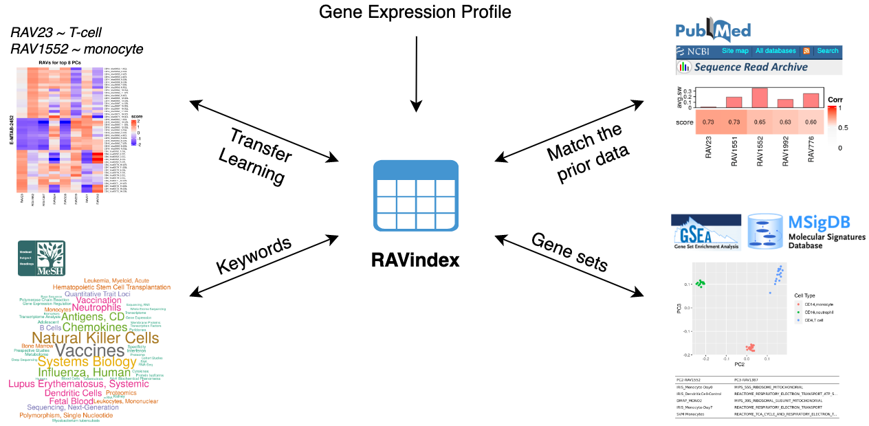
What kinds of information can you access through RAV?

GenomicSuperSignature connects different public databases and prior information through RAVmodel, creating the knowledge graph illustrated below. Through RAVs, you can access and explore the knowledge graph from multiple entry points such as gene expression profiles, publications, study metadata, keywords in MeSH terms and gene sets.

MeSH terms in wordcloud

You can draw a wordcloud with the enriched MeSH terms of RAVs. Based on the heatmap table above, three RAVs (2538, 1139, and 884) show the high validation scores with the positive average silhouette widths, so we draw wordclouds of those RAVs using drawWordcloud function. You need to provide RAVmodel and the index of the RAV you are interested in.

Index of validated RAVs can be easily collected using validatedSingatures function, which outputs the validated index based on num.out, PC from dataset (whichPC) or any *Cutoff arguments in the same way as heatmapTable. Here, we choose the top 3 RAVs with the average silhouette width above 0, which will returns RAV2538, RAV1139, and RAV884 as we discussed above.

validated_ind <- validatedSignatures(val_all, RAVmodel, num.out = 3, 
                                     swCutoff = 0, indexOnly = TRUE)
validated_ind

And we plot the wordcloud of those three RAVs.

set.seed(1) # only if you want to reproduce identical display of the same words
drawWordcloud(RAVmodel, validated_ind[1])
drawWordcloud(RAVmodel, validated_ind[2])
drawWordcloud(RAVmodel, validated_ind[3])

GSEA

Associated gene sets of validated RAV

You can directly access the GSEA outputs for each RAV using annotateRAV function. Based on the wordclouds, RAV1139 seems to be associated with B-cell.

annotateRAV(RAVmodel, validated_ind[2]) # RAV1139

If you want to check the enriched pathways for multiple RAVs, use subsetEnrichedPathways function instead.

subsetEnrichedPathways(RAVmodel, validated_ind[2], include_nes = TRUE)

subsetEnrichedPathways(RAVmodel, validated_ind, include_nes = TRUE)

Search enriched pathways through keyword

You can also find the RAVs annotated with the keyword-containing pathways using findSignature function. Without the k argument, this function outputs a data frame with two columns: the number of RAVs (Freq column) with the different numbers of keyword-containing, enriched pathways (# of keyword-containing pathways column).

Here, we used the keyword, "Bcell".

findSignature(RAVmodel, "Bcell")

There are two RAVs with five keyword-containing pathways (row 6). We can check which RAVs they are.

findSignature(RAVmodel, "Bcell", k = 5)

Enriched pathways are ordered by NES and you can check the rank of any keyword- containing pathways using findKeywordInRAV.

findKeywordInRAV(RAVmodel, "Bcell", ind = 695)

You can check all enriched pathways of RAV using subsetEnrichedPathways function. If both=TRUE, both the top and bottom enriched pathways will be printed.

## Chosen based on validation/MeSH terms
subsetEnrichedPathways(RAVmodel, ind = validated_ind[2], n = 3, both = TRUE)

## Chosen based on enriched pathways
subsetEnrichedPathways(RAVmodel, ind = 695, n = 3, both = TRUE)
subsetEnrichedPathways(RAVmodel, ind = 953, n = 3, both = TRUE)
subsetEnrichedPathways(RAVmodel, ind = 1994, n = 3, both = TRUE)

Related prior studies

You can find the prior studies related to a given RAV using findStudiesInCluster function.

findStudiesInCluster(RAVmodel, validated_ind[2])

You can easily extract the study name with the studyTitle=TRUE parameter.

findStudiesInCluster(RAVmodel, validated_ind[2], studyTitle = TRUE)

Session Info

sessionInfo()

shbrief/GenomicSuperSignature documentation built on May 3, 2023, 10:07 p.m.