In shbrief/PCAGenomicSignatures: Interpretation of RNA-seq experiments through robust, efficient comparison to public databases

knitr::opts_chunk$set(
  collapse = TRUE, comment = "#>" 
)

Citing GenomicSuperSignature

Please cite GenomicSuperSignature as follows:

Oh, S., Geistlinger, L., Ramos, M. et al. GenomicSuperSignature facilitates interpretation of RNA-seq experiments through robust, efficient comparison to public databases. Nat Commun 13, 3695 (2022). https://doi.org/10.1038/s41467-022-31411-3

Setup

Install and load package

if (!require("BiocManager"))
    install.packages("BiocManager")
BiocManager::install("GenomicSuperSignature")

library(GenomicSuperSignature)

Download RAVmodel

You can download GenomicSuperSignature from Google Cloud bucket using GenomicSuperSignature::getModel function. Currently available models are built from top 20 PCs of 536 studies (containing 44,890 samples) containing 13,934 common genes from each of 536 study's top 90% varying genes based on their study-level standard deviation. There are two versions of this RAVmodel annotated with different gene sets for GSEA: MSigDB C2 (C2) and three priors from PLIER package (PLIERpriors). In this vignette, we are showing the C2 annotated model.

Note that the first interactive run of this code, you will be asked to allow R to create a cache directory. The model file will be stored there and subsequent calls to getModel will read from the cache.

RAVmodel <- getModel("C2", load=TRUE)

Content of RAVmodel

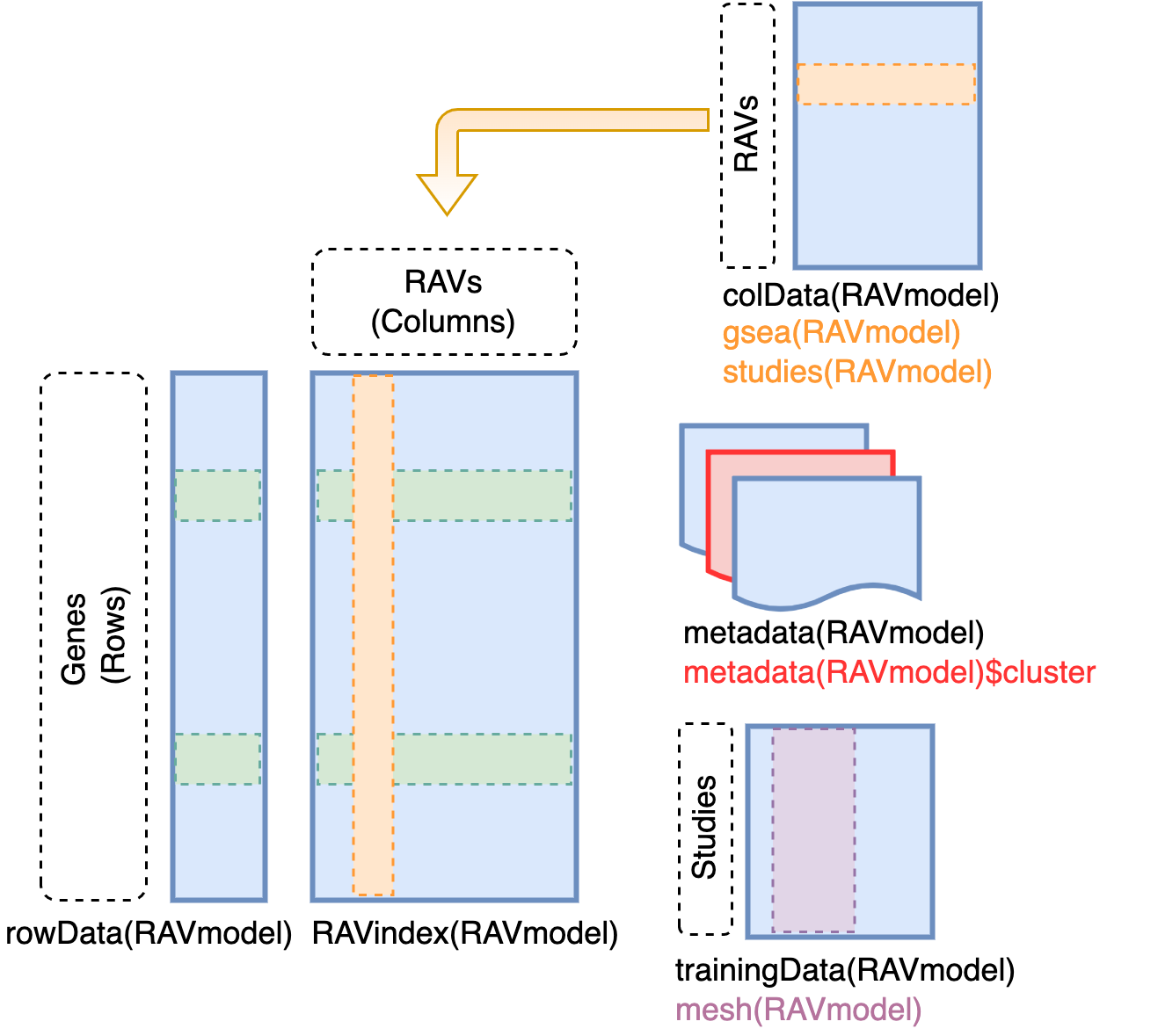
RAVindex is a matrix containing genes in rows and RAVs in columns. colData slot provides the information on each RAVs, such as GSEA annotation and studies involved in each cluster. metadata slot stores model construction information. trainingData slot contains the information on individual studies in training dataset, such as MeSH terms assigned to each study.

RAVmodel

version(RAVmodel)
geneSets(RAVmodel)

RAVindex

Replicable Axis of Variation (RAV) index is the main component of GenomicSuperSignature. It serves as an index connecting new datasets and the existing database. You can access it through GenomicSuperSignature::RAVindex (equivalent of SummarizedExperiment::assay). Rows are genes and columns are RAVs.

Here, RAVmodel consists of 13,934 genes and 4,764 RAVs.

class(RAVindex(RAVmodel))
dim(RAVindex(RAVmodel))
RAVindex(RAVmodel)[1:4, 1:4]

Metadata for RAVmodel

Metadata slot of RAVmodel contains information related to the model building.

names(metadata(RAVmodel))

• cluster : cluster membership of each PCs from the training dataset
• size : an integer vector with the length of clusters, containing the number of PCs in each cluster
• k : the number of all clusters in the given RAVmodel
• n : the number of top PCs kept from each study in the training dataset
• geneSets : the name of gene sets used for GSEA annotation
• MeSH_freq : the frequency of MeSH terms associated with the training dataset. MeSH terms like 'Humans' and 'RNA-seq' are top ranked (which is very expected) because the training dataset of this model is Human RNA sequencing data.
• updateNote : a brief note on the given model's specification
• version : the version of the given model

head(metadata(RAVmodel)$cluster)
head(metadata(RAVmodel)$size)
metadata(RAVmodel)$k
metadata(RAVmodel)$n
geneSets(RAVmodel)
head(metadata(RAVmodel)$MeSH_freq)
updateNote(RAVmodel)  
metadata(RAVmodel)$version

Studies in each RAV

You can find which studies are in each cluster using studies method. Output is a list with the length of clusters, where each element is a character vector containing the name of studies in each cluster.

length(studies(RAVmodel))
studies(RAVmodel)[1:3]

You can check which PC from different studies are in RAVs using PCinRAV.

PCinRAV(RAVmodel, 2)

Silhouette width for each RAV

Silhouette width ranges from -1 to 1 for each cluster. Typically, it is interpreted as follows:
- Values close to 1 suggest that the observation is well matched to the assigned cluster
- Values close to 0 suggest that the observation is borderline matched between two clusters
- Values close to -1 suggest that the observations may be assigned to the wrong cluster

For RAVmodel, the average silhouette width of each cluster is a quality control measure and suggested as a secondary reference to choose proper RAVs, following validation score.

x <- silhouetteWidth(RAVmodel)
head(x)   # average silhouette width of the first 6 RAVs

GSEA on each RAV

Pre-processed GSEA results on each RAV are stored in RAVmodel and can be accessed through gsea function.

class(gsea(RAVmodel))
class(gsea(RAVmodel)[[1]])
length(gsea(RAVmodel))
gsea(RAVmodel)[1]

MeSH terms for each study

You can find MeSH terms associated with each study using mesh method. Output is a list with the length of studies used for training. Each element of this output list is a data frame containing the assigned MeSH terms and the detail of them. The last column bagOfWords is the frequency of the MeSH term in the whole training dataset.

length(mesh(RAVmodel))
mesh(RAVmodel)[1]

PCA summary for each study

PCA summary of each study can be accessed through PCAsummary method. Output is a list with the length of studies, where each element is a matrix containing PCA summary results: standard deviation (SD), variance explained by each PC (Variance), and the cumulative variance explained (Cumulative).

length(PCAsummary(RAVmodel))
PCAsummary(RAVmodel)[1]

Other relevant code

The workflow to build the RAVmodel is available from https://github.com/shbrief/model_building which is archived in Zenodo with the identifier https://doi.org/10.5281/zenodo.6496552. All analyses presented in the GenomicSuperSignatures manuscript are reproducible using code accessible from https://github.com/shbrief/GenomicSuperSignaturePaper/ and archived in Zenodo with the identifier [https://doi.org/10.5281/zenodo.6496612].

Session Info

sessionInfo()

shbrief/PCAGenomicSignatures documentation built on May 3, 2023, 11:21 a.m.