In timjmiller/wham: Woods Hole Assessment Model (WHAM)

knitr::opts_chunk$set(
  collapse = TRUE,
  comment = "#>"
)
#wham.dir <- find.package("wham")
#knitr::opts_knit$set(root.dir = file.path(wham.dir,"extdata"))
is.repo <- try(pkgload::load_all(compile=FALSE)) #this is needed to build the vignettes without the new version of wham installed.
if(is.character(is.repo)) library(wham) #not building webpage
#note that if plots are not yet pushed to the repo, they will not show up in the html.
wham.dir <- find.package("wham")

In this vignette we walk through an example using the wham (WHAM = Woods Hole Assessment Model) package to run a state-space age-structured stock assessment model. WHAM is a generalization of code written for Miller et al. (2016) and Xu et al. (2018), and in this example we apply WHAM to the same stock, Southern New England / Mid-Atlantic Yellowtail Flounder.

Here we assume you already have wham installed. If not, see the Introduction. This is the 3rd wham example, which builds off model m5 from example 2:

• full state-space model (numbers-at-age are random effects for all ages, NAA_re = list(sigma='rec+1',cor='iid'))

• logistic normal age compositions (age_comp = "logistic-normal-pool0")

• Beverton-Holt recruitment (recruit_model = 3)

• Cold Pool Index (CPI) fit as an AR1 process (ecov$process_model = "ar1")

• CPI has a "limiting" (carrying capacity, Iles and Beverton (1998)) effect on recruitment (ecov$where = "recruit", ecov$how = 2)

In example 3, we demonstrate how to project/forecast WHAM models using the project_wham() function options for handling

• fishing mortality / catch (use last F, use average F, use $F_{SPR}$, use $F_{MSY}$, specify F, specify catch) and the

• environmental covariate (continue ecov process, use last ecov, use average ecov, specify ecov).

1. Load data

Open R and load the wham package:

library(wham)

For a clean, runnable .R script, look at ex3_projections.R in the example_scripts folder of the wham package. You can run this entire example script with:

wham.dir <- find.package("wham")
source(file.path(wham.dir, "example_scripts", "ex3_projections.R"))

Let's create a directory for this analysis:

# choose a location to save output, otherwise will be saved in working directory
write.dir <- "choose/where/to/save/output" # need to change e.g., tempdir(check=TRUE)
dir.create(write.dir)
setwd(write.dir)

We need the same data files as in example 2. Read in ex2_SNEMAYT.dat and CPI.csv:

wham.dir <- find.package("wham")
asap3 <- read_asap3_dat(file.path(wham.dir,"extdata","ex2_SNEMAYT.dat"))
env.dat <- read.csv(file.path(wham.dir,"extdata","CPI.csv"), header=T)

2. Specify model

Setup model m5 from example 2:

• full state-space model (numbers-at-age are random effects for all ages, NAA_re = list(sigma='rec+1',cor='iid'))

• logistic normal age compositions (age_comp = "logistic-normal-pool0")

• Beverton-Holt recruitment (recruit_model = 3)

• Cold Pool Index (CPI) fit as an AR1 process (ecov$process_model = "ar1")

• CPI has a "controlling" (density-independent mortality, Iles and Beverton (1998)) effect on recruitment (ecov$where = "recruit", ecov$how = 1)

env <- list(
  label = "CPI",
  mean = as.matrix(env.dat$CPI), # CPI observations
  logsigma = as.matrix(log(env.dat$CPI_sigma)), # CPI standard error is given/fixed as data
  year = env.dat$Year,
  use_obs = matrix(1, ncol=1, nrow=dim(env.dat)[1]), # use all obs (=1)
  process_model = "ar1", # fit CPI as AR1 process
  recruitment_how = matrix("limiting-lag-1-linear")) # limiting (carrying capacity), CPI in year t affects recruitment in year t+1

input <- prepare_wham_input(asap3, recruit_model = 3,
                            model_name = "Ex 3: Projections",
                            ecov = env,
                            NAA_re = list(sigma="rec+1", cor="iid"),
                            age_comp = "logistic-normal-pool0") # logistic normal pool 0 obs

# selectivity = logistic, not age-specific
#   2 pars per block instead of n.ages
#   sel pars of indices 4/5 fixed at 1.5, 0.1 (neg phase in .dat file)
input$par$logit_selpars[1:4,7:8] <- 0 # original code started selpars at 0 (last 2 rows are fixed)

3. Fit the model without projections

You have two options for projecting a WHAM model:

1. Fit model without projections and then add projections afterward

# don't run
mod <- fit_wham(input) # default do.proj=FALSE
mod_proj <- project_wham(mod)

1. Add projections with initial model fit (do.proj = TRUE)

# don't run
mod_proj <- fit_wham(input, do.proj = TRUE)

The two code blocks above are equivalent; when do.proj = TRUE, fit_wham() fits the model without projections and then calls project_wham() to add them. In this example we choose option #1 because we are going to add several different projections to the same model, mod. We will save each projected model in a list, mod_proj.

# run
mod <- fit_wham(input)
saveRDS(mod, file="m5.rds") # save unprojected model

4. Add projections to fit model

Projection options are specifed using the proj.opts input to project_wham(). The default settings are to project 3 years (n.yrs = 3), use average maturity-, weight-, and natural mortality-at-age from last 5 model years to calculate reference points (avg.yrs), use fishing mortality in the last model year (use.last.F = TRUE), and continue the ecov process model (cont.ecov = TRUE). These options are also described in the project_wham() help page.

 # save projected models in a list
mod_proj <- list()

# default settings spelled out
mod_proj[[1]] <- project_wham(mod, proj.opts=list(n.yrs=3, use.last.F=TRUE, use.avg.F=FALSE, 
  use.FXSPR=FALSE, use.FMSY=FALSE, proj.F=NULL, proj.catch=NULL, avg.yrs=NULL, 
  cont.ecov=TRUE, use.last.ecov=FALSE, avg.ecov.yrs=NULL, proj.ecov=NULL, cont.Mre=NULL, 
  avg.rec.yrs=NULL, percentFXSPR=100, percentFMSY=100))

# equivalent
# mod_proj[[1]] <- project_wham(mod)

WHAM implements four options for handling the environmental covariate(s) in the projections. Exactly one of these must be specified in proj.opts if ecov is in the model:

• (Default) Continue the ecov process model (e.g. random walk, AR1). Set cont.ecov = TRUE. WHAM will estimate the ecov process in the projection years (i.e. continue the random walk / AR1 process).

• Use last year ecov. Set use.last.ecov = TRUE. WHAM will use ecov value from the terminal year of the population model for projections.

• Use average ecov. Provide avg.yrs.ecov, a vector specifying which years to average over the environmental covariate(s) for projections.

• Specify ecov. Provide proj.ecov, a matrix of user-specified environmental covariate(s) to use for projections. Dimensions must be the number of projection years (proj.opts$n.yrs) x the number of ecovs (ncols(ecov$mean)).

Note that for all options, if the original model fit the ecov in years beyond the population model, WHAM will use these already-fit ecov values for the projections. If the ecov model extended at least proj.opts$n.yrs years beyond the population model, then none of the above need be specified.

# 5 years, use average ecov from 1992-1996
mod_proj[[2]] <- project_wham(mod, proj.opts=list(n.yrs=5, use.last.F=TRUE, use.avg.F=FALSE,
              use.FXSPR=FALSE, proj.F=NULL, proj.catch=NULL, avg.yrs=NULL,
              cont.ecov=FALSE, use.last.ecov=FALSE, avg.ecov.yrs=1992:1996, proj.ecov=NULL))
# equivalent
# mod_proj[[2]] <- project_wham(mod, proj.opts=list(n.yrs=5, avg.ecov.yrs=1992:1996))

# 5 years, use ecov from last year (2011)
mod_proj[[3]] <- project_wham(mod, proj.opts=list(n.yrs=5, use.last.F=TRUE, use.avg.F=FALSE,
              use.FXSPR=FALSE, proj.F=NULL, proj.catch=NULL, avg.yrs=NULL,
              cont.ecov=FALSE, use.last.ecov=TRUE, avg.ecov.yrs=NULL, proj.ecov=NULL))
# equivalent
# mod_proj[[3]] <- project_wham(mod, proj.opts=list(n.yrs=5, use.last.ecov=TRUE))

# 5 years, specify high CPI ~ 0.5
# note: again, need 5 years of CPI because in general, the lag of the CPI effect may not be known (no effect) or it may differ by effect on various population attributes,
mod_proj[[4]] <- project_wham(mod, proj.opts=list(n.yrs=5, use.last.F=TRUE, use.avg.F=FALSE,
              use.FXSPR=FALSE, proj.F=NULL, proj.catch=NULL, avg.yrs=NULL,
              cont.ecov=FALSE, use.last.ecov=FALSE, avg.ecov.yrs=NULL, 
              proj.ecov=matrix(c(0.5,0.7,0.4,0.5,0.55),ncol=1)))
# equivalent
# mod_proj[[4]] <- project_wham(mod, proj.opts=list(n.yrs=5, proj.ecov=matrix(c(0.5,0.7,0.4,0.5,0.55),ncol=1)))

# 5 years, specify low CPI ~ -1.5
# note: again, need 5 years of CPI because in general, the lag of the CPI effect may not be known (no effect) or it may differ by effect on various population attributes,
mod_proj[[5]] <- project_wham(mod, proj.opts=list(n.yrs=5, use.last.F=TRUE, use.avg.F=FALSE,
              use.FXSPR=FALSE, proj.F=NULL, proj.catch=NULL, avg.yrs=NULL,
              cont.ecov=FALSE, use.last.ecov=FALSE, avg.ecov.yrs=NULL, 
              proj.ecov=matrix(c(-1.6,-1.3,-1,-1.2,-1.25),ncol=1)))

# equivalent
# mod_proj[[5]] <- project_wham(mod, proj.opts=list(n.yrs=5, proj.ecov=matrix(c(-1.6,-1.3,-1,-1.2,-1.25),ncol=1)))

WHAM implements six options for handling fishing mortality in the projections. Exactly one of these must be specified in proj.opts:

• (Default) Use last year F. Set use.last.F = TRUE. WHAM will use F in the terminal model year for projections.

• Use average F. Set use.avg.F = TRUE. WHAM will use F averaged over proj.opts$avg.yrs for projections (as is done for M-, maturity-, and weight-at-age).

• Use F at X% SPR. Set use.FXSPR = TRUE. WHAM will calculate and apply F at X% SPR, where X was set by input$data$percentSPR (default = 40%). There is also a percentFXSPR

• Specify F. Provide proj.F, an F vector with length = proj.opts$n.yrs.

• Specify catch. Provide proj.catch, a vector of aggregate catch with length = proj.opts$n.yrs. WHAM will calculate F across fleets to apply the specified catch.

• Use FMSY. Set use.FMSY = TRUE. WHAM will calculate and apply F at MSY. There is a check to make sure that a stock-recruit model is assumed and, if not, F at X% SPR is used instead.

# 5 years, specify catch
mod_proj[[6]] <- project_wham(mod, proj.opts=list(n.yrs=5, use.last.F=FALSE, use.avg.F=FALSE,
              use.FXSPR=FALSE, proj.F=NULL, proj.catch=c(10, 2000, 1000, 3000, 20), avg.yrs=NULL,
              cont.ecov=TRUE, use.last.ecov=FALSE, avg.ecov.yrs=NULL, proj.ecov=NULL))
# equivalent
# mod_proj[[6]] <- project_wham(mod, proj.opts=list(n.yrs=5, proj.catch=c(10, 2000, 1000, 3000, 20)))

# 5 years, specify F
mod_proj[[7]] <- project_wham(mod, proj.opts=list(n.yrs=5, use.last.F=FALSE, use.avg.F=FALSE,
              use.FXSPR=FALSE, proj.F=c(0.001, 1, 0.5, .1, .2), proj.catch=NULL, avg.yrs=NULL,
              cont.ecov=TRUE, use.last.ecov=FALSE, avg.ecov.yrs=NULL, proj.ecov=NULL))
# equivalent
# mod_proj[[7]] <- project_wham(mod, proj.opts=list(n.yrs=5, proj.F=c(0.001, 1, 0.5, .1, .2)))

# 5 years, use FXSPR
mod_proj[[8]] <- project_wham(mod, proj.opts=list(n.yrs=5, use.last.F=FALSE, use.avg.F=FALSE,
              use.FXSPR=TRUE, proj.F=NULL, proj.catch=NULL, avg.yrs=NULL,
              cont.ecov=TRUE, use.last.ecov=FALSE, avg.ecov.yrs=NULL, proj.ecov=NULL))
# equivalent
# mod_proj[[8]] <- project_wham(mod, proj.opts=list(n.yrs=5, use.FXSPR=TRUE))

# 3 years, use avg F (avg.yrs defaults to last 5 years, 2007-2011)
mod_proj[[9]] <- project_wham(mod, proj.opts=list(n.yrs=3, use.last.F=FALSE, use.avg.F=TRUE,
              use.FXSPR=FALSE, proj.F=NULL, proj.catch=NULL, avg.yrs=NULL,
              cont.ecov=TRUE, use.last.ecov=FALSE, avg.ecov.yrs=NULL, proj.ecov=NULL))
# equivalent
# mod_proj[[9]] <- project_wham(mod, proj.opts=list(use.avg.F=TRUE))

# 10 years, use avg F 1992-1996
mod_proj[[10]] <- project_wham(mod, proj.opts=list(n.yrs=10, use.last.F=FALSE, use.avg.F=TRUE,
              use.FXSPR=FALSE, proj.F=NULL, proj.catch=NULL, avg.yrs=1992:1996,
              cont.ecov=TRUE, use.last.ecov=FALSE, avg.ecov.yrs=NULL, proj.ecov=NULL))
# equivalent
# mod_proj[[10]] <- project_wham(mod, proj.opts=list(n.yrs=10, use.avg.F=TRUE, avg.yrs=1992:1996))

# 5 years, use $F_{MSY}$
mod_proj[[11]] <- project_wham(mod, proj.opts=list(n.yrs=5, use.last.F=FALSE, use.avg.F=FALSE,
              use.FMSY=TRUE, proj.F=NULL, proj.catch=NULL, avg.yrs=NULL,
              cont.ecov=TRUE, use.last.ecov=FALSE, avg.ecov.yrs=NULL, proj.ecov=NULL))

Save projected models

saveRDS(mod_proj, file="m5_proj.rds")

5. Compare projections

The models with projections are evaluated to obtain optimized random effects but they do not need to be refitted with projections added because the observations and marginal likelihood do not change. However, we can confirm that the NLL is the same for all projected models (within some tolerance).

#data(vign3_nlls) #not needed. data are available without this call
#data(vign3_nll_proj)
#data(vign3_nll_orig)

mod$opt$obj # original model NLL

vign3_nll_orig

nll_proj <-  sapply(mod_proj, function(x) x$fn()) # projected models marginal NLL
#round(nll_proj - mod$opt$obj, 6) # difference between original and projected models' NLL
nll_proj - mod$opt$obj # difference between original and projected models' NLL

vign3_nll_proj - vign3_nll_orig

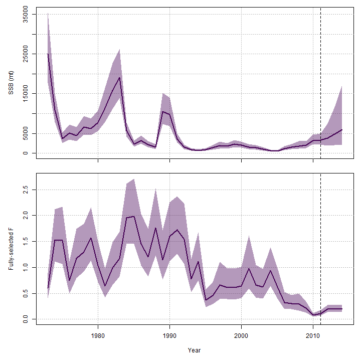
Now let's plot results from each of the projected models.

for(m in 1:length(mod_proj)){
  plot_wham_output(mod_proj[[m]], dir.main=file.path(write.dir,paste0("proj_",m)))
}

6. Results

Projected CPI

{ width=30% }{ width=30% }{ width=30% }

{ width=30% }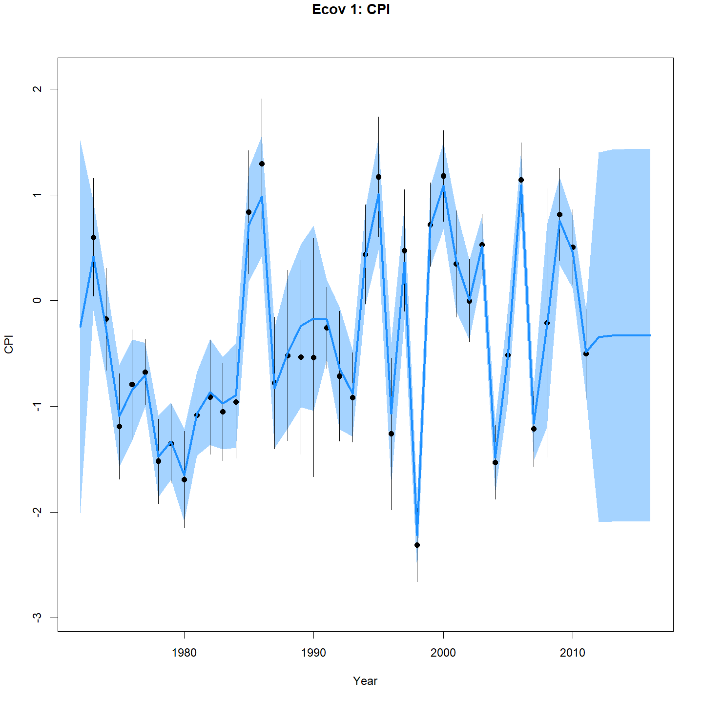{ width=30% }

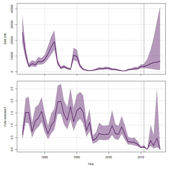
Projected F / catch

{ width=30% }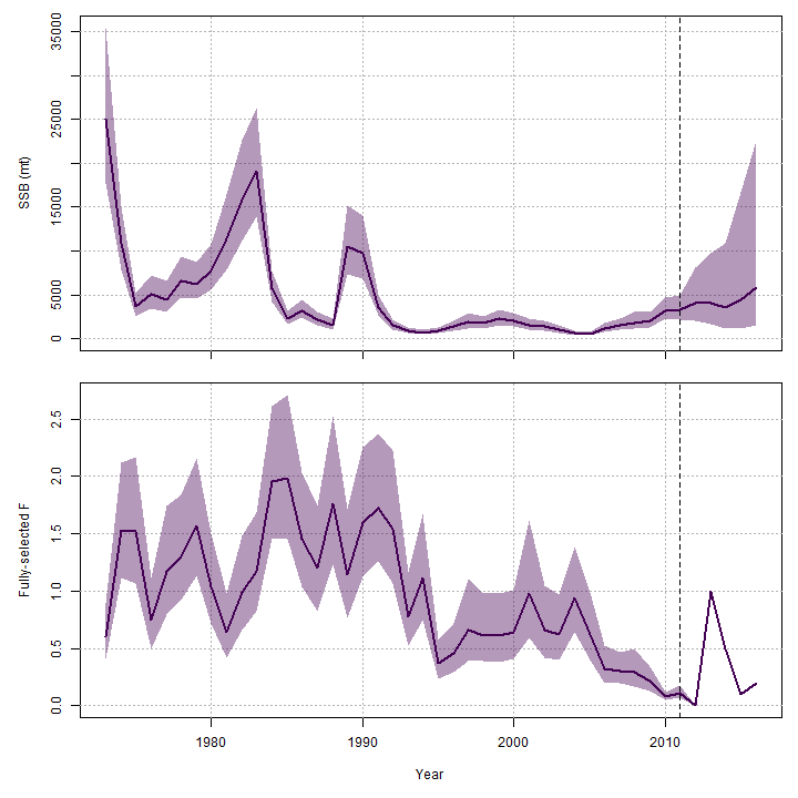{ width=30% }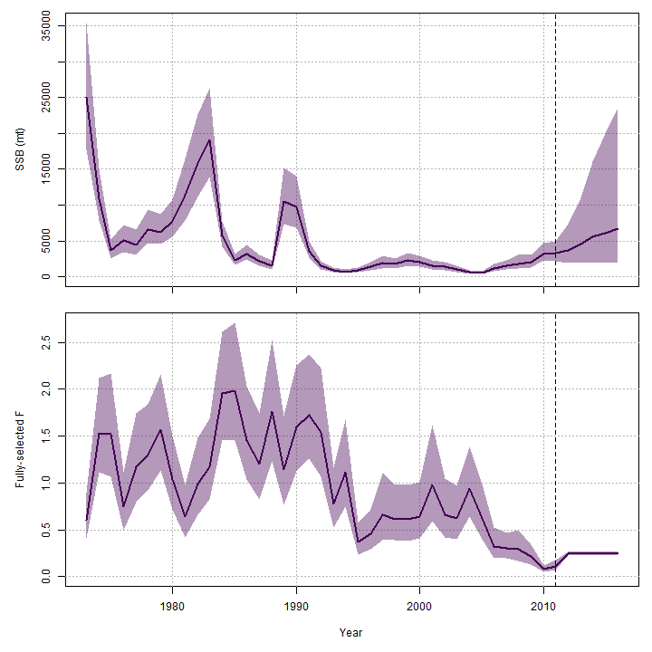{ width=30% }

{ width=30% }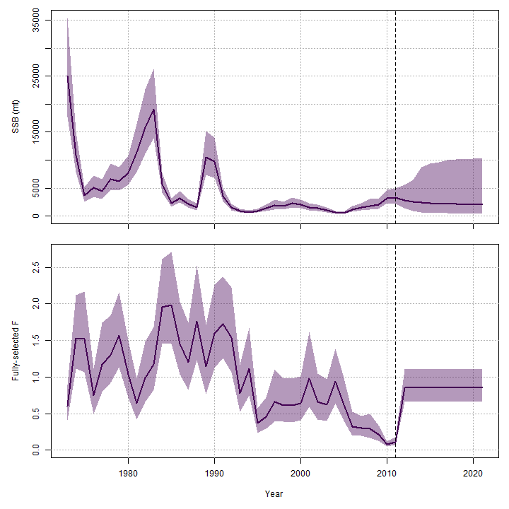{ width=30% }

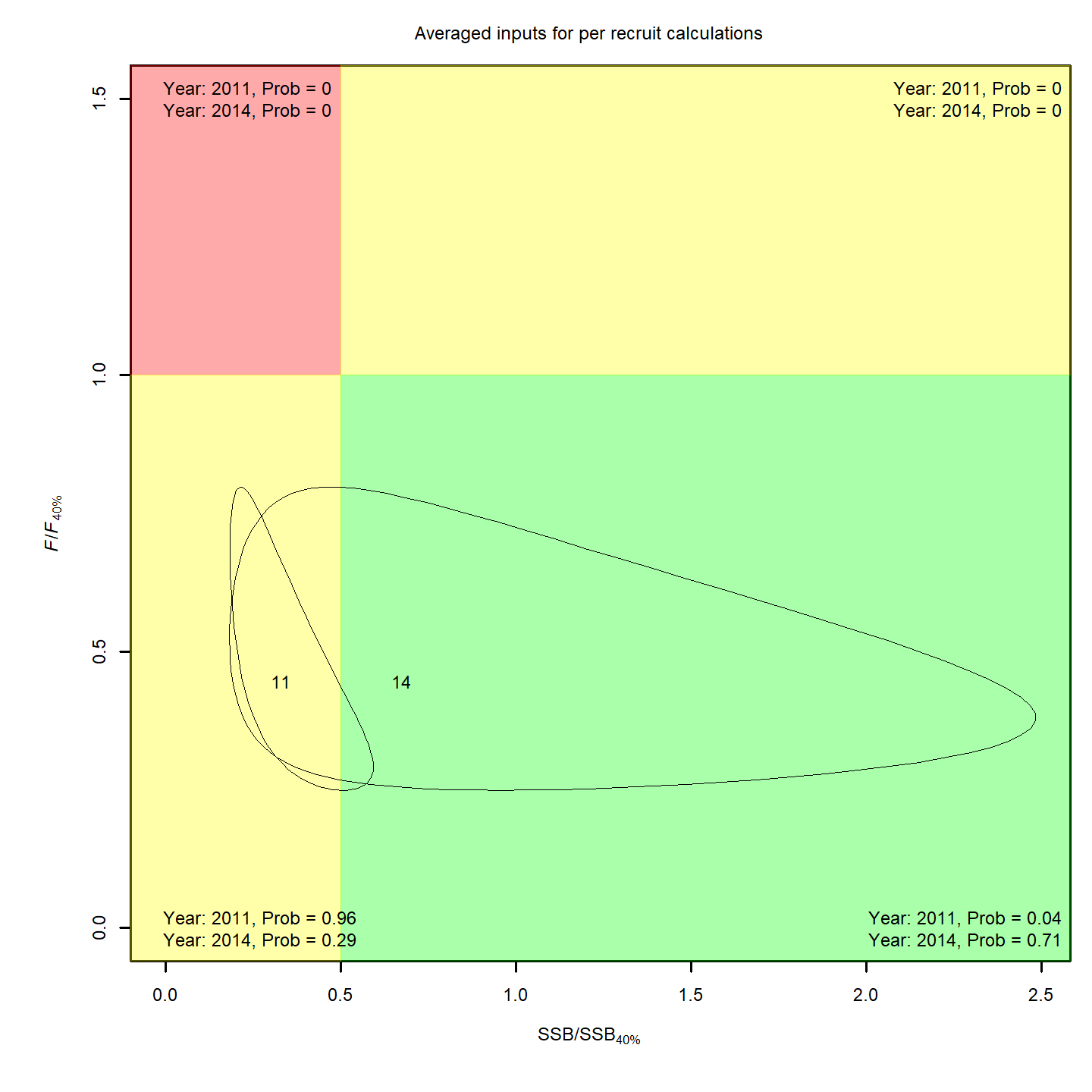
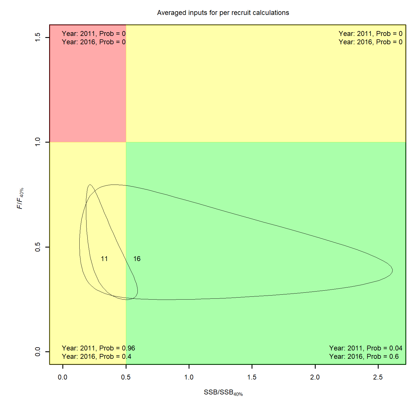
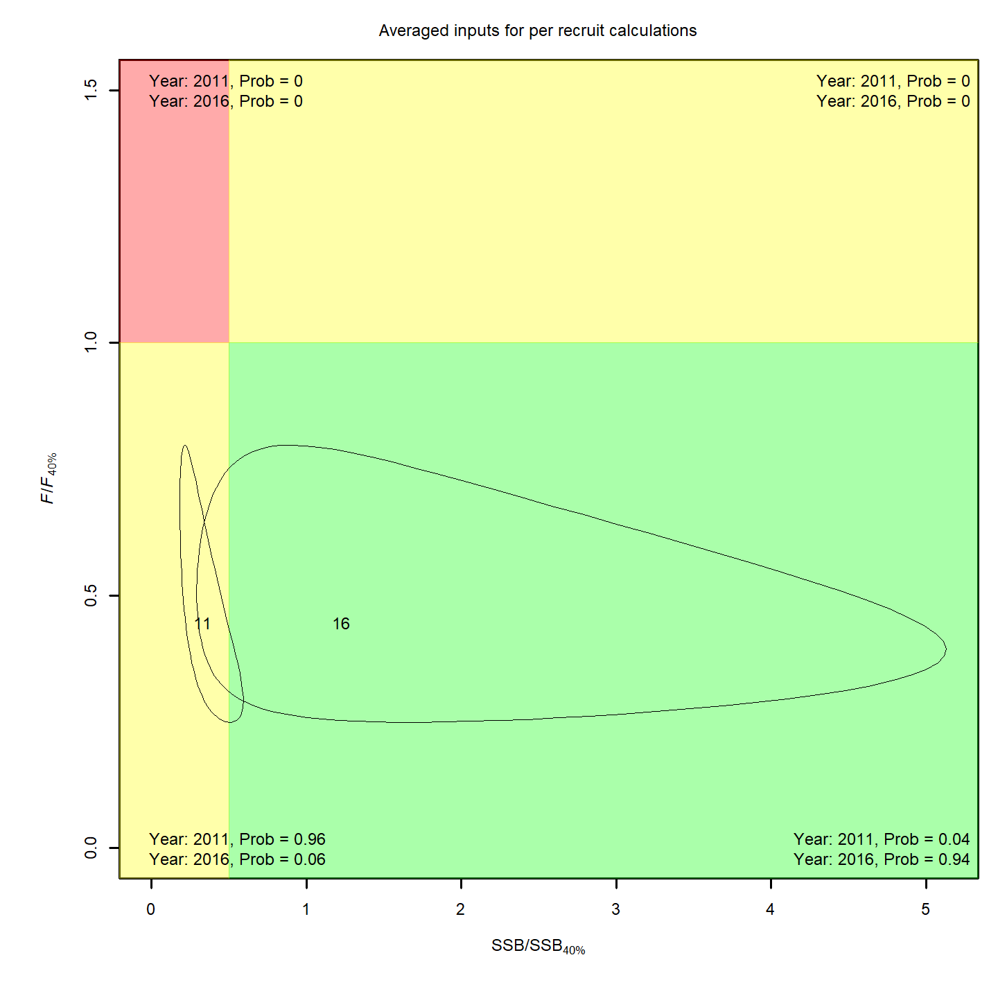
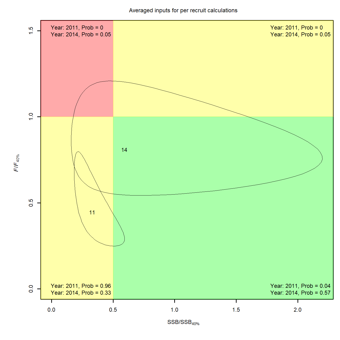
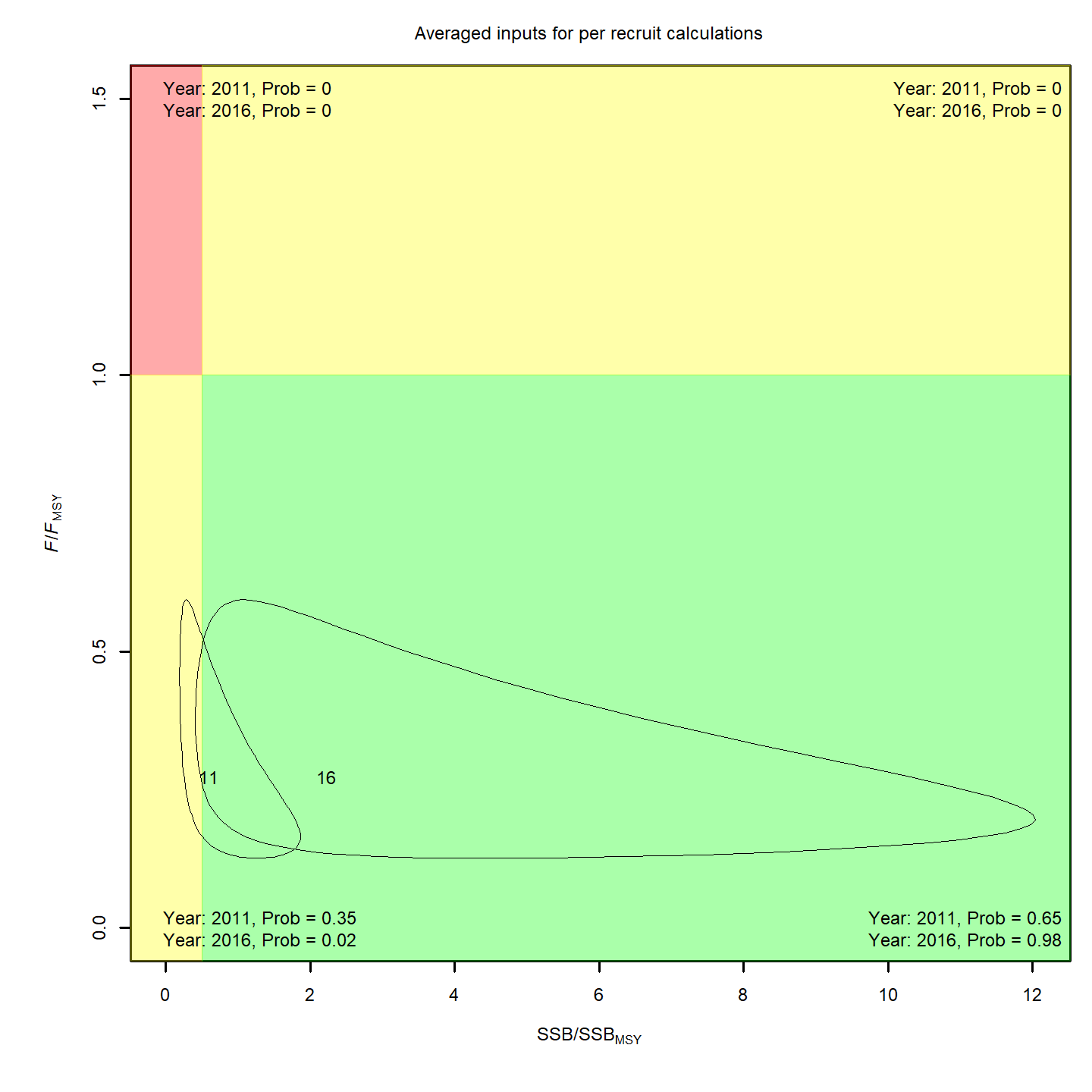
Stock status

In the stock status (Kobe) plots of the projected models using 40% spawning potential ratio for reference points, the final model year is in bold and the final projected year is not bold.

{ width=45% }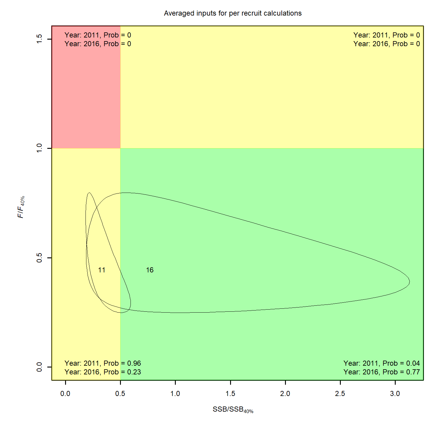{ width=45% }

{ width=45% }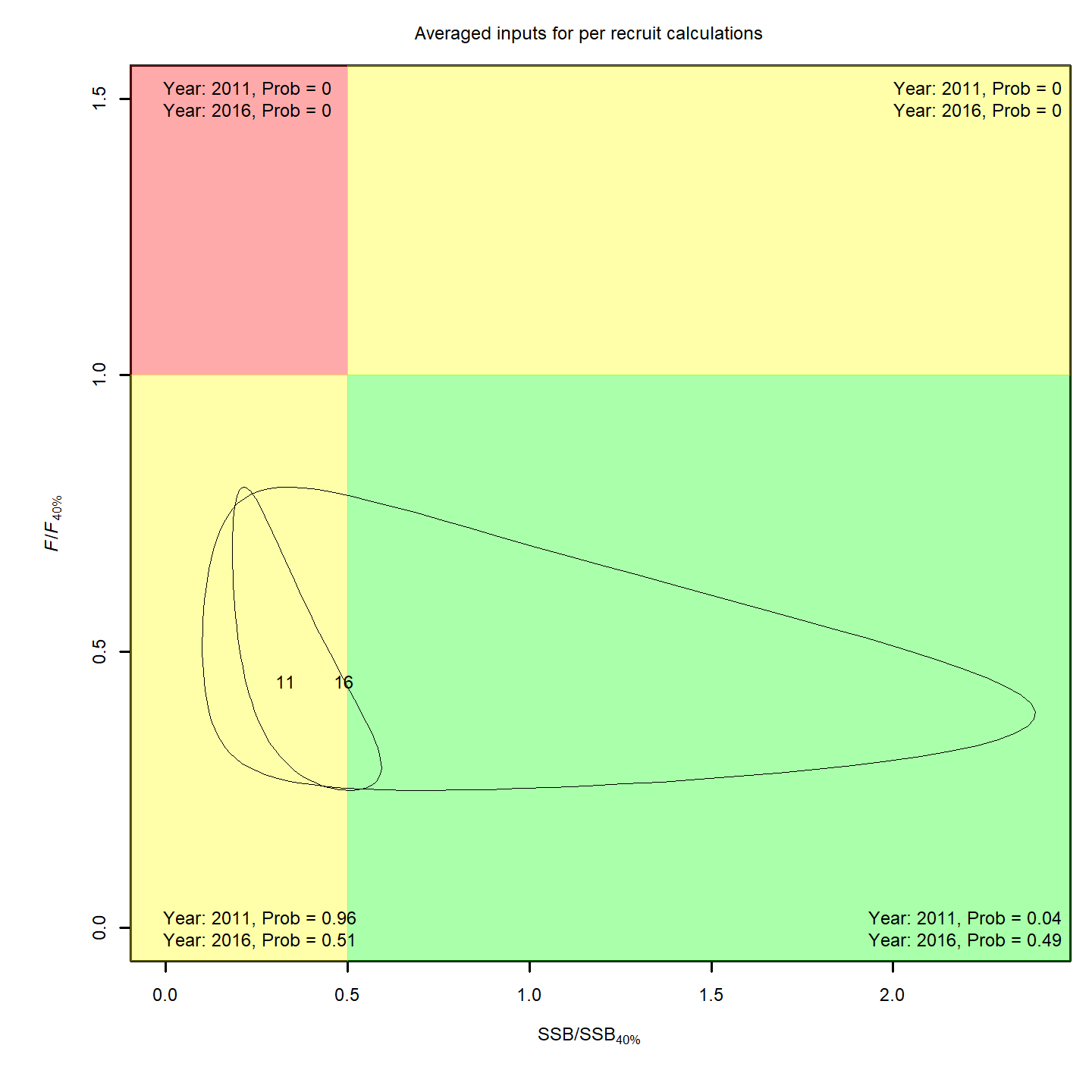{ width=45% }

{ width=45% }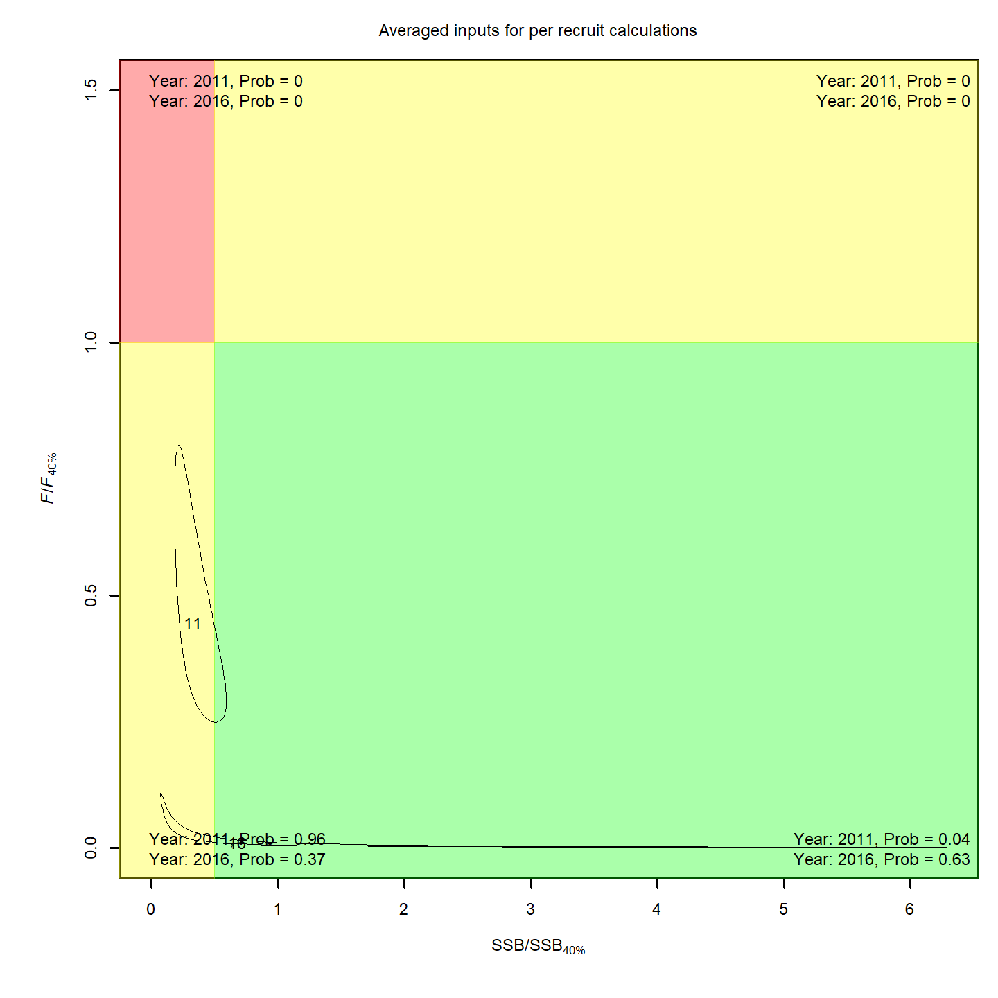{ width=45% }

{ width=45% }{ width=45% }

{ width=45% }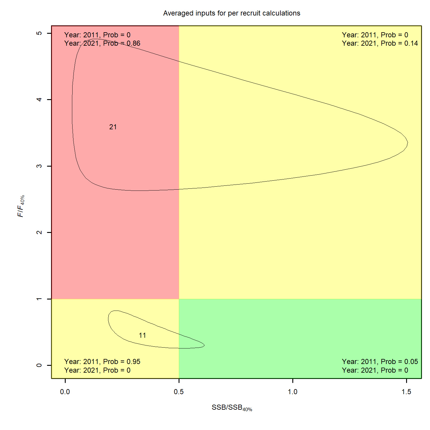{ width=45% }

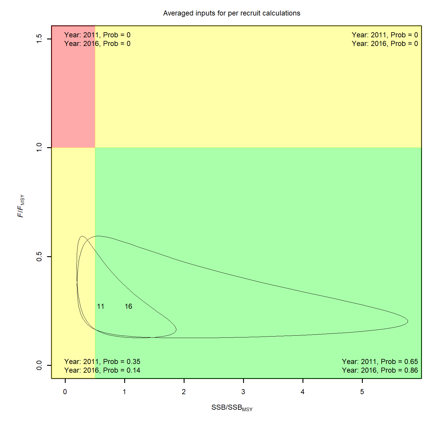
We can compare with the same plots that use MSY-based reference points.

{ width=45% }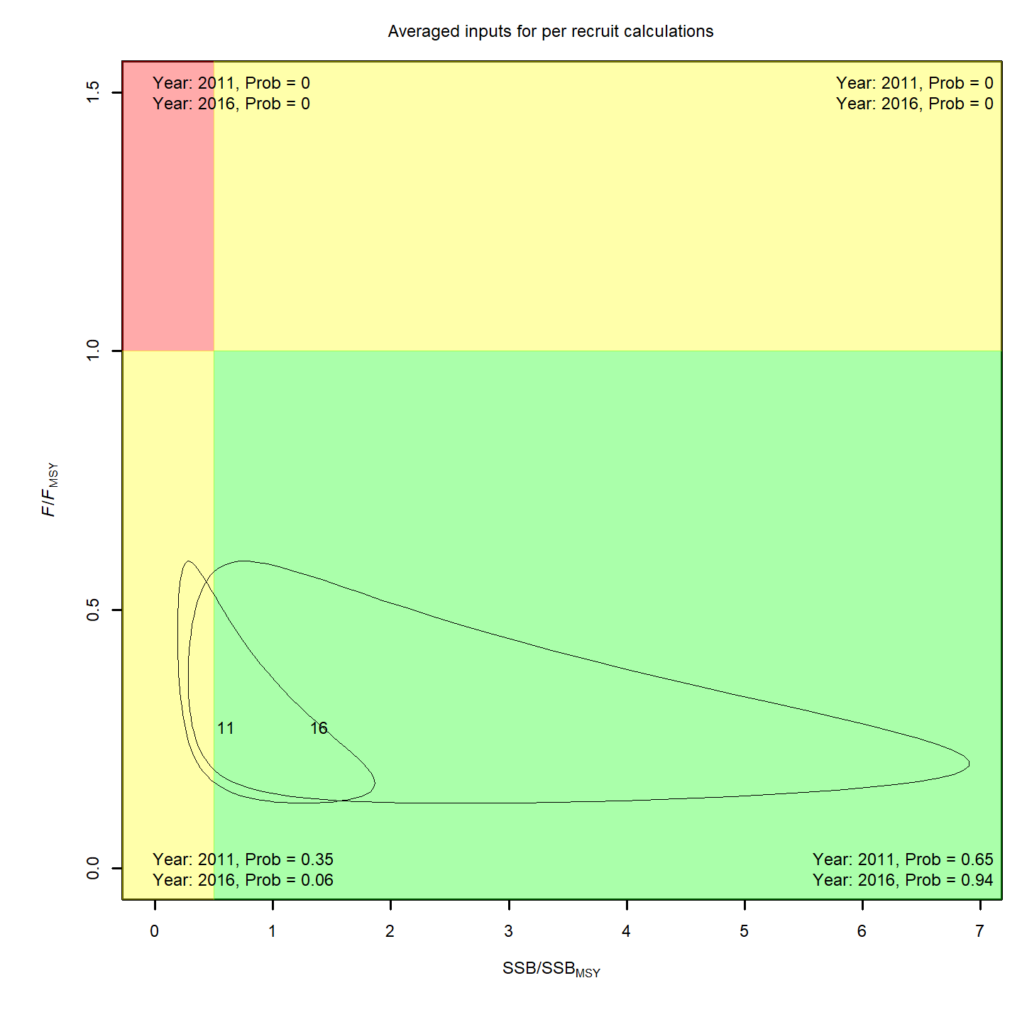{ width=45% }

{ width=45% }{ width=45% }

{ width=45% }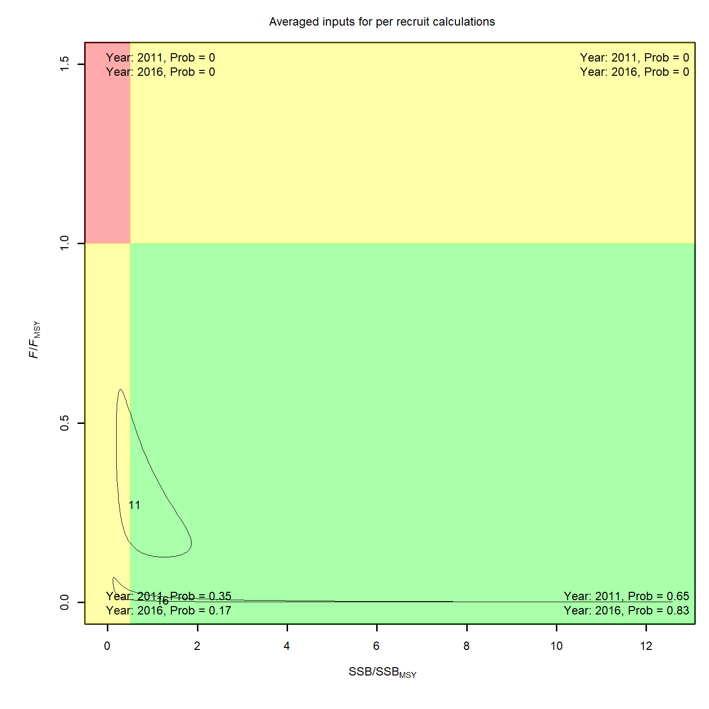{ width=45% }

{ width=45% }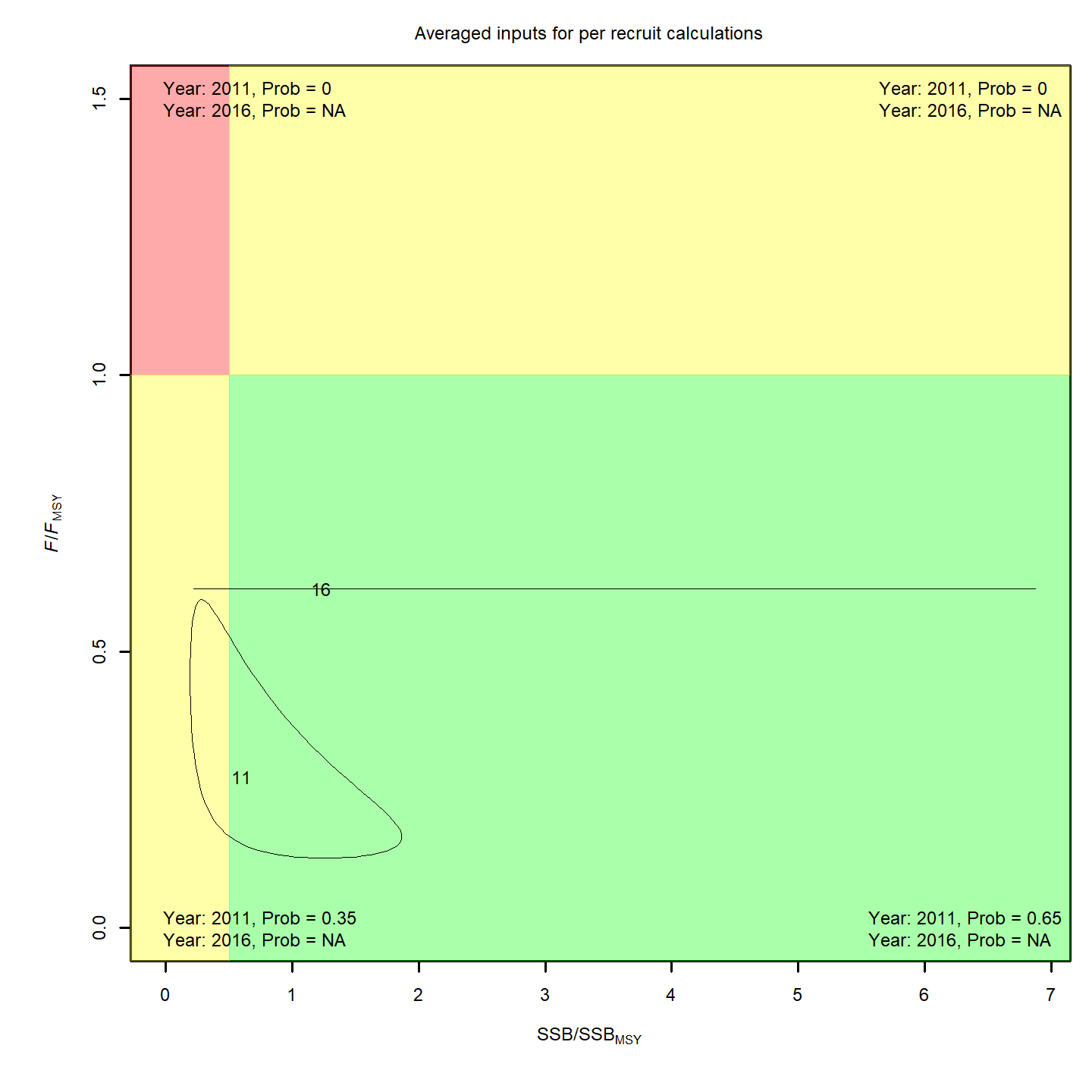{ width=45% }

{ width=45% }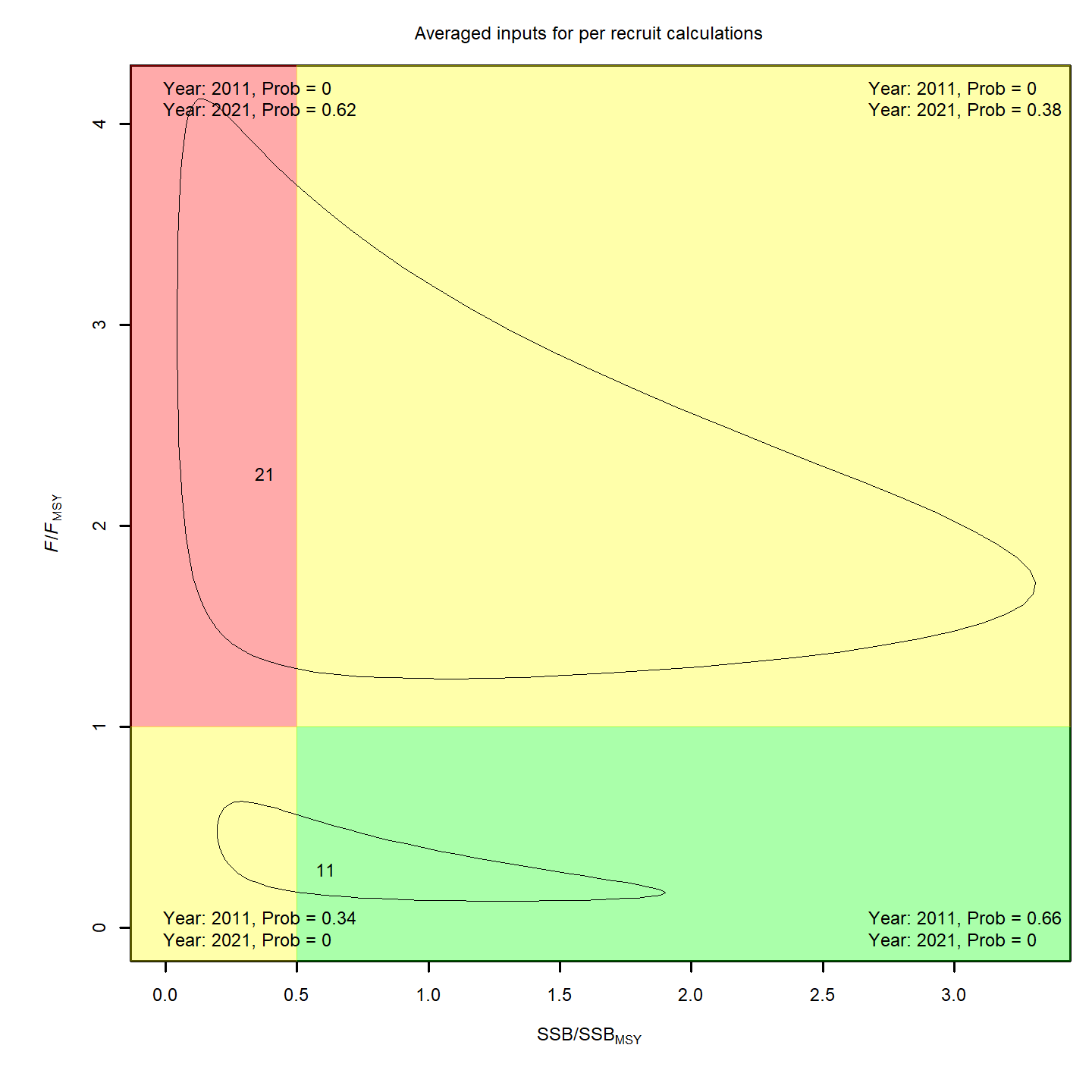{ width=45% }

timjmiller/wham documentation built on Feb. 4, 2025, 10:31 p.m.