In timjmiller/wham: Woods Hole Assessment Model (WHAM)

knitr::opts_chunk$set(
  collapse = TRUE,
  comment = "#>"
)
#wham.dir <- find.package("wham")
#knitr::opts_knit$set(root.dir = file.path(wham.dir,"extdata"))
is.repo <- try(pkgload::load_all(compile=FALSE)) #this is needed to build the vignettes without the new version of wham installed.
if(is.character(is.repo)) library(wham) #not building webpage
#note that if plots are not yet pushed to the repo, they will not show up in the html.
wham.dir <- find.package("wham")
library(tidyverse)
library(viridis)
library(ggplot2)
library(wham)

This is the 9th WHAM example. We assume you already have wham installed and are relatively familiar with the package. If not, read the Introduction and Tutorial.

In this vignette we show how to calculate retrospective predictions, by peeling x years of data, re-fitting models, and then projecting each peel y years. Although this can be done for any variable, we demonstrate how to do so for recruitment, as in Fig. 4 of Xu et al. (2018). We use the same data and model setup as for m3 and m5 from example 2.

1. Load WHAM and other useful packages

# devtools::install_github("timjmiller/wham", dependencies=TRUE)
library(wham)
library(tidyverse)
library(viridis)
library(ggplot2)

Create a directory for this analysis:

# choose a location to save output, otherwise will be saved in working directory
write.dir <- "choose/where/to/save/output"
dir.create(write.dir)
setwd(write.dir)

We need the same data files as in example 2. Let's copy ex2_SNEMAYT.dat and CPI.csv to our analysis directory:

wham.dir <- find.package("wham")
file.copy(from=file.path(wham.dir,"extdata","ex2_SNEMAYT.dat"), to=write.dir, overwrite=TRUE)
file.copy(from=file.path(wham.dir,"extdata","CPI.csv"), to=write.dir, overwrite=TRUE)
asap3 <- read_asap3_dat("ex2_SNEMAYT.dat")
env.dat <- read.csv("CPI.csv", header=T)

2. Specify models

Setup models m5 (with CPI effect on recruitment) and m3 (no CPI effect on recruitment) from example 2:

full state-space model (numbers-at-age are random effects for all ages, NAA_re = list(sigma='rec+1',cor='iid'))
logistic normal age compositions (age_comp = "logistic-normal-pool0")
Beverton-Holt recruitment (recruit_model = 3)
Cold Pool Index (CPI) fit as an AR1 process (ecov$process_model = "ar1")
CPI has a "limiting" (e.g. carrying capacity, Iles and Beverton (1998)) effect on recruitment (ecov$where = "recruit", ecov$how = 2)

env <- list(
  label = "CPI",
  mean = as.matrix(env.dat$CPI), # CPI observations
  logsigma = as.matrix(log(env.dat$CPI_sigma)), # CPI standard error is given/fixed as data
  year = env.dat$Year,
  use_obs = matrix(1, ncol=1, nrow=dim(env.dat)[1]), # use all obs (=1)
  lag = 1, # CPI in year t affects recruitment in year t+1
  process_model = "ar1", # fit CPI as AR1 process
  where = "recruit", # CPI affects recruitment
  how = NA) # fill in by model in loop

# 2 models, with and without CPI effect on recruitment (both fit CPI data to compare AIC)
# Model  Recruit_mod  Ecov_mod     Ecov_how
#    m1     Bev-Holt       ar1        ---
#    m2     Bev-Holt       ar1     Limiting
df.mods <- data.frame(Model = c("m1","m2"), Ecov_how = c(0,2), stringsAsFactors=FALSE)
n.mods <- dim(df.mods)[1]
df.mods

3. Fit the models

for(m in 1:n.mods){
    env$how = df.mods$Ecov_how[m]
    input <- prepare_wham_input(asap3, recruit_model = 3,
                                model_name = df.mods$Model[m],
                                ecov = env,
                                NAA_re = list(sigma="rec+1", cor="iid"),
                                age_comp = "logistic-normal-pool0") # logistic normal pool 0 obs
    input$par$logit_selpars[1:4,7:8] <- 0

    # fit model
    mod <- fit_wham(input, do.retro=F, do.osa=F)
    saveRDS(mod, file=paste0(df.mods$Model[m],".rds"))
    plot_wham_output(mod=mod, dir.main=file.path(getwd(),df.mods$Model[m]), out.type='png')
}

4. Look at convergence and diagnostics

mod.list <- file.path(write.dir,paste0("m",1:n.mods,".rds"))
mods <- lapply(mod.list, readRDS)
ok_sdrep = sapply(mods, function(x) if(x$na_sdrep==FALSE & !is.na(x$na_sdrep)) 1 else 0)
df.mods$conv <- sapply(mods, function(x) x$opt$convergence == 0) # 0 means opt converged
df.mods$pdHess <- as.logical(ok_sdrep)

Compare model output - they are pretty similar.

names(mods) <- c("m1 (no CPI)","m2 (CPI)")
res <- compare_wham_models(mods, fdir=write.dir, do.table=F, plot.opts=list(kobe.prob=FALSE))

5. Run retrospective predictions

For each model, peel 3-15 years of data and re-fit the model using retro(), and then project each peel 3 years by calling project_wham(). These projections are done with F = 0 and continuing the CPI AR1 process model (without new observations). You can specify alternative options for the projections using $proj.opts (see project_wham() and Ex 3: Projections).

n.yrs.peel <- 15
n.yrs.proj <- 3
for(m in 1:n.mods){
    mods[[m]]$peels <- retro(mods[[m]], ran = unique(names(mods[[m]]$env$par[mods[[m]]$env$random])), n.peels=n.yrs.peel, save.input = T)
    for(p in 3:n.yrs.peel) mods[[m]]$peels[[p]] <- project_wham(mods[[m]]$peels[[p]], proj.opts = list(n.yrs = n.yrs.proj, proj.F=rep(0.001,n.yrs.proj)))
}

6. Plot retrospective predictions of recruitment

Here is a function to extract and plot the retrospective predictions of recruitment from each model. It can easily be modified to extract other variables of interest, e.g. SSB or F.

plot_retro_pred_R <- function(mods, peels=3:n.yrs.peel, n.yrs.proj=n.yrs.proj){
    df <- data.frame(matrix(NA, nrow=0, ncol=6))
    colnames(df) <- c("Year","Model","Peel","Recruitment","termyr")
    for(m in 1:length(mods)){
        for(p in peels){
            tmp <- read_wham_fit(mods[[m]]$peels[[p]])
            df <- rbind(df, data.frame(Year=tail(tmp$years_full, n.yrs.proj+1),
                                        Model=names(mods)[m],
                                        Peel=p,
                                        Recruitment=tail(exp(tmp$log_NAA[,1]), n.yrs.proj+1),
                                        termyr=c(1,rep(0,n.yrs.proj))))
        }
        # get full model fit, "peel 0"
        tmp <- read_wham_fit(mods[[m]])
        df <- rbind(df, data.frame(Year=tmp$years,
                                    Model=names(mods)[m],
                                    Peel=0,
                                    Recruitment=exp(tmp$log_NAA[1:length(tmp$years),1]),
                                    termyr=0))
    }

    df <- filter(df, Year > 1990)
    df$Model <- factor(df$Model, levels=names(mods), labels=names(mods))
    df$Year <- as.integer(df$Year) 
    df$Peel <- factor(df$Peel)
    dfpts <- filter(df, termyr==1)

    cols <- c("black", viridis_pal(option="plasma")(length(levels(df$Peel))-1))
    g <- ggplot(df, aes(x=Year, y=Recruitment, linetype=Model, color=Peel, fill=Peel, group=interaction(Model,Peel))) + 
          geom_line(linewidth=1) +
          geom_point(data=dfpts, color='black', size=2, pch=21) +
          scale_x_continuous(expand=c(0.01,0.01)) + # breaks=scales::breaks_extended(5)
          scale_colour_manual(values=cols) +
          scale_fill_manual(values=cols) +
          guides(color = "none", fill="none") +
          scale_y_continuous(expand=c(0.01,0.01), limits = c(0,NA), labels=fancy_scientific) +
          theme_bw() +
          theme(legend.position=c(.9,.9), legend.box.margin = margin(0,0,0,0), legend.margin = margin(0,0,0,0))
    return(g)
}

plot_retro_pred_R(mods, peels=3:n.yrs.peel, n.yrs.proj=n.yrs.proj)
ggsave(file.path(write.dir,"retro_pred_R.png"), device='png', width=8, height=5, units='in')

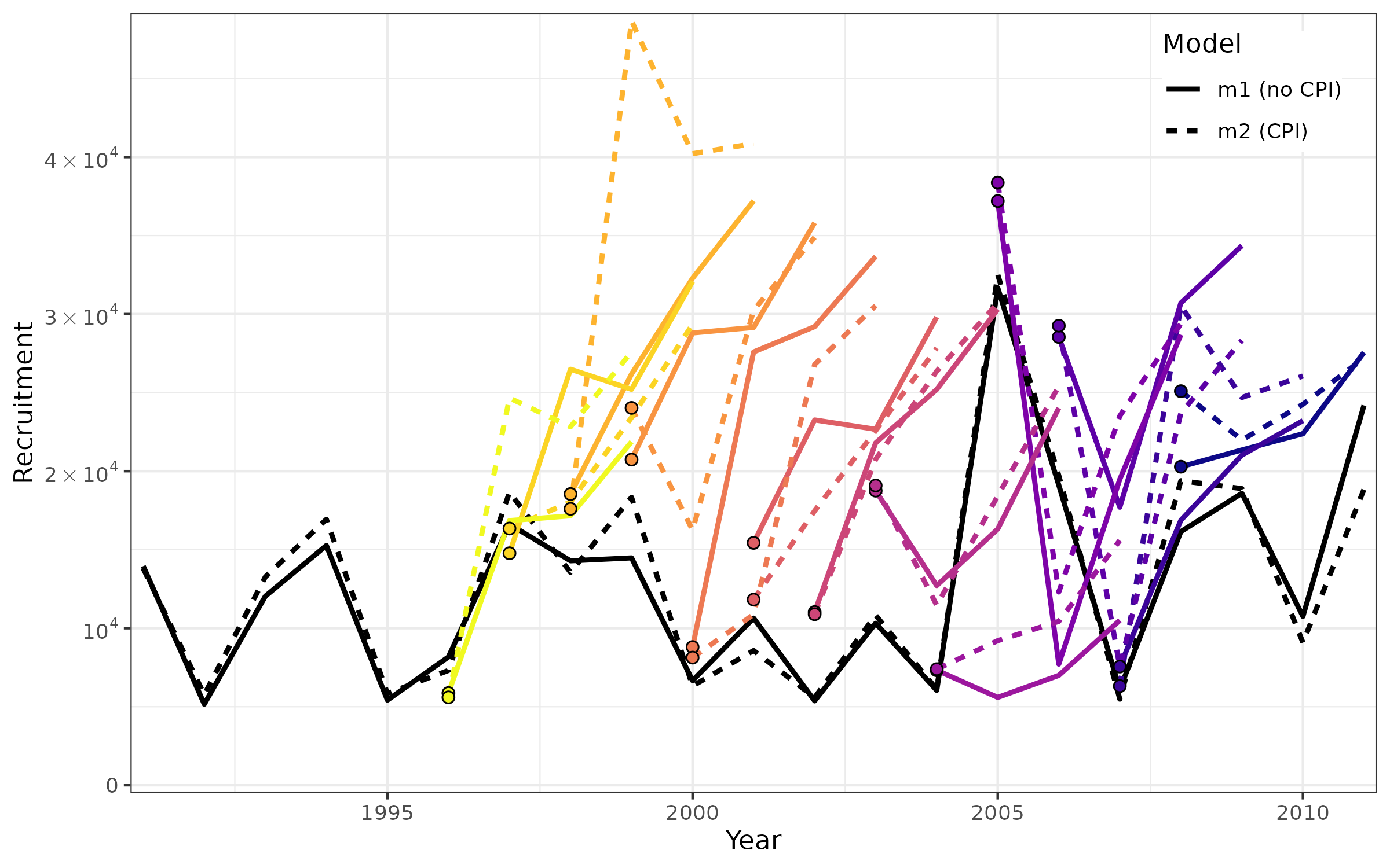
The two black lines represent the "true" recruitment from each model, i.e., the recruitment estimates when fitting to the full data. Points and lines are colored by peel from yellow (1996) to dark blue (2008). The points are terminal year recruitment estimates and lines are projected recruitment (3 years).

{ width=95% }