README.md

In audrina/pcclust: PCA Analysis and Visualization for Clustering

Pcclust

Overview

Pcclust is a versatile and comprehensive R package for PCA analysis and visualization, specifically designed to tailor PC selection for optimizing downstream cluster analysis.

The analysis pipeline employs 2 metrics to quantify the cluster quality that is obtained when using different combinations of PCs. Using the R mclust package it calculates Bayesian information criterion (BIC) and maximum log likelihood for Gaussian mixture models (GMM) in order to determine the subset of PCs containing the most significant cluster structure.

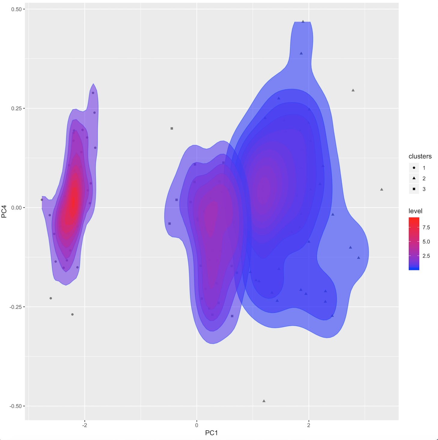
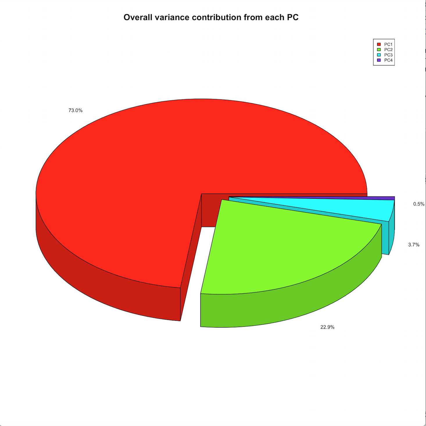
The comprehensive visualization component of the pipeline then produces several informative PCA graphics, using the optimal choice of PCs for clustering as determined in the analysis stages of the pipeline, and includes the following: Baseline PCA visualizations: a standard 2-component PCA plot, density plot, and variance contribution pie chart. 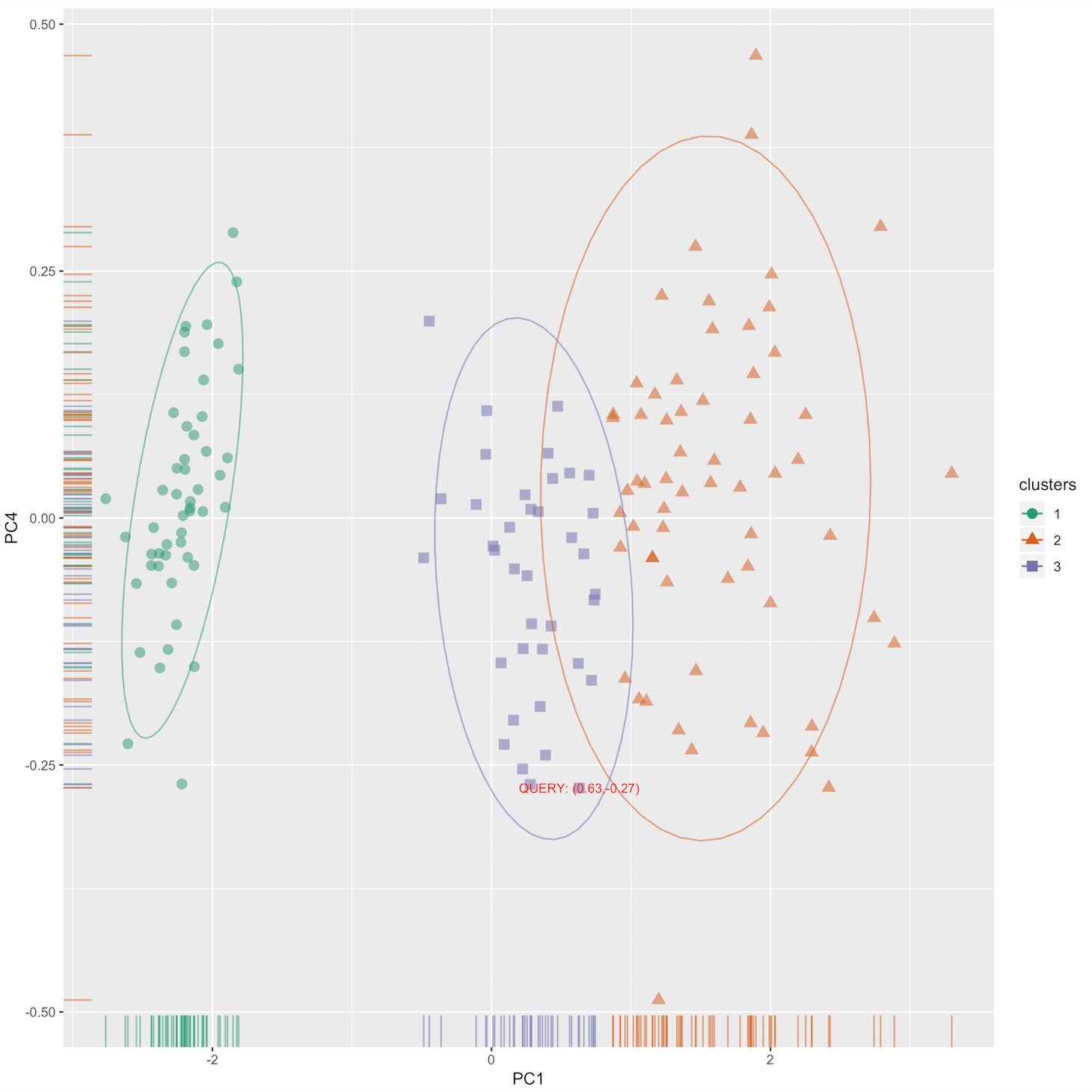Additional functionality enabling one to "zoom-in" on a specific query point which will produce sample-specific metadata: * A standard 2-component PCA plot labeled with the query point. 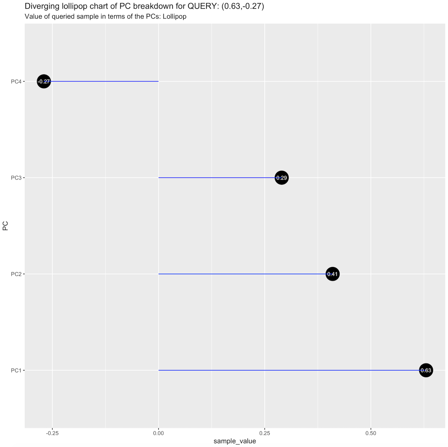* A diverging lollipop chart showing the PC breakdown for the query sample. 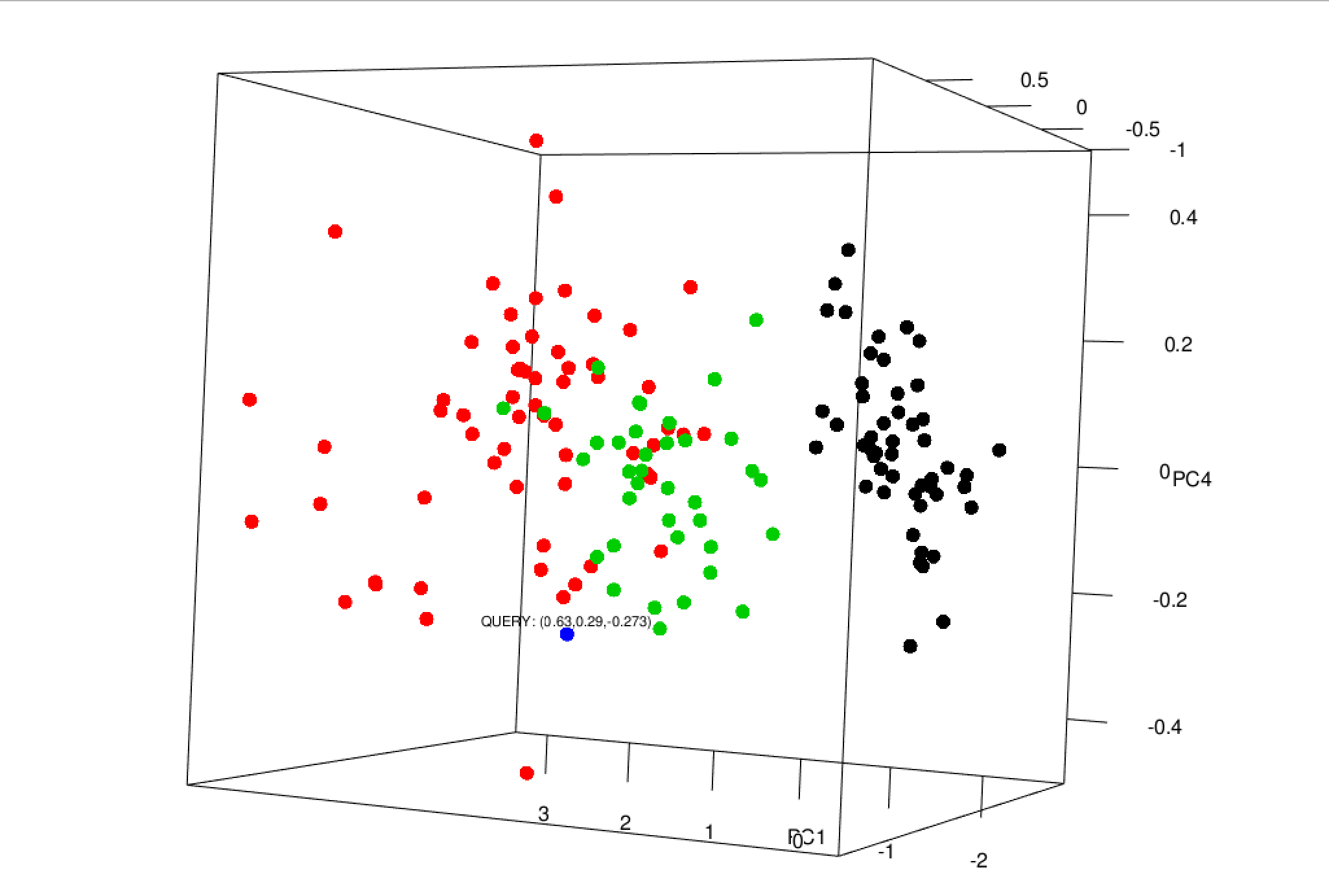* An interactive PCA plot showing the location of the query point in 3D space.

Dependencies

• R packages: mclust, ggplot2, rio, plotrix, rgl, car

General usage

Pcclust will accept any numeric multidimensional matrix or data frame as input to the analysis pipeline; optionally accepting an appropriate file that is in a format supported by rio.

Pipeline workflow instructions

To execute the pipeline in sequence, follow these steps (uses the Iris dataset as a PoC):

library(devtools)
install_github("audrina/pcclust")
library(pcclust)

# 1. validate and load data
irisCSV <- system.file("extdata", "iris.csv", package = "pcclust")
data <- validateAndLoadData(irisCSV, isFile = TRUE)

# 2. run PCA
pcObj <- prcomp(data)
pcData <- pcObj$x

# 3. execute automated PC filtering to get the best optimal PC subset
iterationResults <- executePCFiltering(pcData)

bestPCSet <- iterationResults[[length(iterationResults)]] # optimal set corresponds to last iteration

optimalModel <- determineOptimalModel(bestPCSet)

clusters <- optimalModel$classification # predictions made by optimal model

# 4. generate baseline visualizations

# returns a path to the ouput folder "pcclust_visualization"
# outDir is the current working directory by default.
out <- visualizePCA(bestPCSet, clusters, pcObj, outDir = ".") 

# 5. query specific points from the optimal PCA plot "optimalPC.svg" in "pcclust_visualization"

# NEW: interactive querying 
runPcclustApp()

x <- 0.5
y <- -0.3

x <- 0
y <- 0

# NOTE: pcclust will always find the nearest neighbor, so queries that are 
# out of range will simply return the max/min for the respective dimensions.

x <- 100 
y <- -100

zoomPC(x, y, pcData, bestPCSet, clusters, iterationResults, out)

Install

library(devtools)
install_github("audrina/pcclust")
library(pcclust)

Sample visualizations

audrina/pcclust documentation built on May 31, 2019, 12:44 a.m.