tab_style: Add custom styles to one or more cells

In gt: Easily Create Presentation-Ready Display Tables

Add custom styles to one or more cells

Description

With tab_style() we can target specific cells and apply styles to them. This is best done in conjunction with the helper functions cell_text(), cell_fill(), and cell_borders(). Currently, this function is focused on the application of styles for HTML output only (as such, other output formats will ignore all tab_style() calls). Using the aforementioned helper functions, here are some of the styles we can apply:

• the background color of the cell (cell_fill(): color)

• the cell's text color, font, and size (cell_text(): color, font, size)

• the text style (cell_text(): style), enabling the use of italics or oblique text.

• the text weight (cell_text(): weight), allowing the use of thin to bold text (the degree of choice is greater with variable fonts)

• the alignment and indentation of text (cell_text(): align and indent)

• the cell borders (cell_borders())

Usage

tab_style(data, style, locations)

Arguments

data	The gt table data object ⁠obj:<gt_tbl>⁠ // required This is the gt table object that is commonly created through use of the gt() function.
style	Style declarations ⁠<style expressions>⁠ // required The styles to use for the cells at the targeted locations. The cell_text(), cell_fill(), and cell_borders() helper functions can be used here to more easily generate valid styles. If using more than one helper function to define styles, all calls must be enclosed in a list(). Custom CSS declarations can be used for HTML output by including a css()-based statement as a list item.
locations	Locations to target <locations expressions> // required The cell or set of cells to be associated with the style. Supplying any of the ⁠cells_*()⁠ helper functions is a useful way to target the location cells that are associated with the styling. These helper functions are: cells_title(), cells_stubhead(), cells_column_spanners(), cells_column_labels(), cells_row_groups(), cells_stub(), cells_body(), cells_summary(), cells_grand_summary(), cells_stub_summary(), cells_stub_grand_summary(), cells_footnotes(), and cells_source_notes(). Additionally, we can enclose several ⁠cells_*()⁠ calls within a list() if we wish to apply styling to different types of locations (e.g., body cells, row group labels, the table title, etc.).

Value

An object of class gt_tbl.

Using from_column() with ⁠cell_*()⁠ styling functions

from_column() can be used with certain arguments of cell_fill() and cell_text(); this allows you to get parameter values from a specified column within the table. This means that body cells targeted for styling could be formatted a little bit differently, using options taken from a column. For cell_fill(), we can use from_column() for its color argument. cell_text() allows the use of from_column() in the following arguments:

• color

• size

• align

• v_align

• style

• weight

• stretch

• decorate

• transform

• whitespace

• indent

Please note that for all of the aforementioned arguments, a from_column() call needs to reference a column that has data of the correct type (this is different for each argument). Additional columns for parameter values can be generated with cols_add() (if not already present). Columns that contain parameter data can also be hidden from final display with cols_hide().

Importantly, a tab_style() call with any use of from_column() within styling expressions must only use cells_body() within locations. This is because we cannot map multiple options taken from a column onto other locations.

Examples

Let's use the exibble dataset to create a simple, two-column gt table (keeping only the num and currency columns). With tab_style() (called twice), we'll selectively add style to the values formatted by fmt_number(). In the style argument of each tab_style() call, we can define multiple types of styling with cell_fill() and cell_text() (enclosed in a list). The cells to be targeted for styling require the use of helpers like cells_body(), which is used here with different columns and rows being targeted.

exibble |>
  dplyr::select(num, currency) |>
  gt() |>
  fmt_number(decimals = 1) |>
  tab_style(
    style = list(
      cell_fill(color = "lightcyan"),
      cell_text(weight = "bold")
      ),
    locations = cells_body(
      columns = num,
      rows = num >= 5000
    )
  ) |>
  tab_style(
    style = list(
      cell_fill(color = "#F9E3D6"),
      cell_text(style = "italic")
      ),
    locations = cells_body(
      columns = currency,
      rows = currency < 100
    )
  )

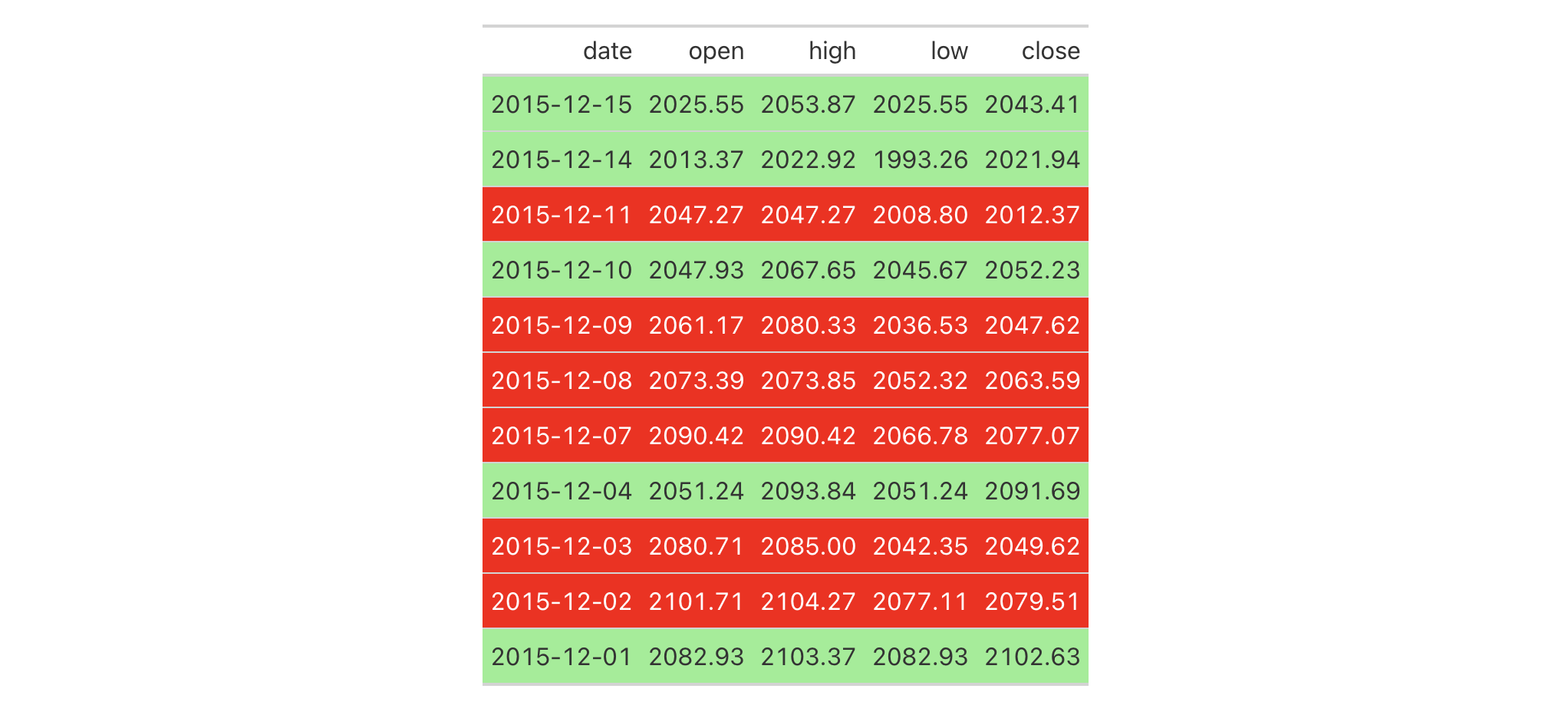
With a subset of the sp500 dataset, we'll create a different gt table. Here, we'll color the background of entire rows of body cells and do so on the basis of value expressions involving the open and close columns.

sp500 |>
  dplyr::filter(
    date >= "2015-12-01" &
    date <= "2015-12-15"
  ) |>
  dplyr::select(-c(adj_close, volume)) |>
  gt() |>
  tab_style(
    style = cell_fill(color = "lightgreen"),
    locations = cells_body(rows = close > open)
  ) |>
  tab_style(
    style = list(
      cell_fill(color = "red"),
      cell_text(color = "white")
      ),
    locations = cells_body(rows = open > close)
  )

With another two-column table based on the exibble dataset, let's create a gt table. First, we'll replace missing values with sub_missing(). Next, we'll add styling to the char column. This styling will be HTML-specific and it will involve (all within a list): (1) a cell_fill() call (to set a "lightcyan" background), and (2) a string containing a CSS style declaration ("font-variant: small-caps;").

exibble |>
  dplyr::select(char, fctr) |>
  gt() |>
  sub_missing() |>
  tab_style(
    style = list(
      cell_fill(color = "lightcyan"),
      "font-variant: small-caps;"
    ),
    locations = cells_body(columns = char)
  )

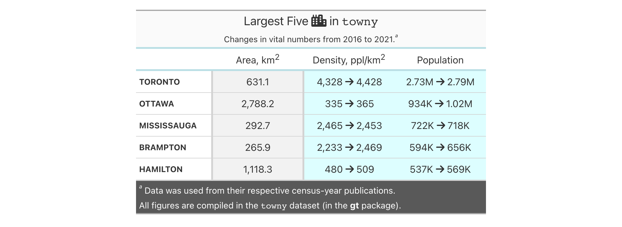
In the following table based on the towny dataset, we'll use a larger number of tab_style() calls with the aim of styling each location available in the table. Over six separate uses of tab_style(), different body cells are styled with background colors, the header and the footer also receive background color fills, borders are applied to a column of body cells and also to the column labels, and, the row labels in the stub receive a custom text treatment.

towny |>
  dplyr::filter(csd_type == "city") |>
  dplyr::select(
    name, land_area_km2, density_2016, density_2021,
    population_2016, population_2021
  ) |>
  dplyr::slice_max(population_2021, n = 5) |>
  gt(rowname_col = "name") |>
  tab_header(
    title = md(paste("Largest Five", fontawesome::fa("city") , "in `towny`")),
    subtitle = "Changes in vital numbers from 2016 to 2021."
  ) |>
  fmt_number(
    columns = starts_with("population"),
    n_sigfig = 3,
    suffixing = TRUE
  ) |>
  fmt_integer(columns = starts_with("density")) |>
  fmt_number(columns = land_area_km2, decimals = 1) |>
  cols_merge(
    columns = starts_with("density"),
    pattern = paste("{1}", fontawesome::fa("arrow-right"), "{2}")
  ) |>
  cols_merge(
    columns = starts_with("population"),
    pattern = paste("{1}", fontawesome::fa("arrow-right"), "{2}")
  ) |>
  cols_label(
    land_area_km2 = md("Area, km^2^"),
    starts_with("density") ~ md("Density, ppl/km^2^"),
    starts_with("population") ~ "Population"
  ) |>
  cols_align(align = "center", columns = -name) |>
  cols_width(
    stub() ~ px(125),
    everything() ~ px(150)
  ) |>
  tab_footnote(
    footnote = "Data was used from their respective census-year publications.",
    locations = cells_title(groups = "subtitle")
  ) |>
  tab_source_note(source_note = md(
    "All figures are compiled in the `towny` dataset (in the **gt** package)."
  )) |>
  opt_footnote_marks(marks = "letters") |>
  tab_style(
    style = list(
      cell_fill(color = "gray95"),
      cell_borders(sides = c("l", "r"), color = "gray50", weight = px(3))
    ),
    locations = cells_body(columns = land_area_km2)
  ) |>
  tab_style(
    style = cell_fill(color = "lightblue" |> adjust_luminance(steps = 2)),
    locations = cells_body(columns = -land_area_km2)
  ) |>
  tab_style(
    style = list(cell_fill(color = "gray35"), cell_text(color = "white")),
    locations = list(cells_footnotes(), cells_source_notes())
  ) |>
  tab_style(
    style = cell_fill(color = "gray98"),
    locations = cells_title()
  ) |>
  tab_style(
    style = cell_text(
      size = "smaller",
      weight = "bold",
      transform = "uppercase"
    ),
    locations = cells_stub()
  ) |>
  tab_style(
    style = cell_borders(
      sides = c("t", "b"),
      color = "powderblue",
      weight = px(3)
    ),
    locations = list(cells_column_labels(), cells_stubhead())
  )

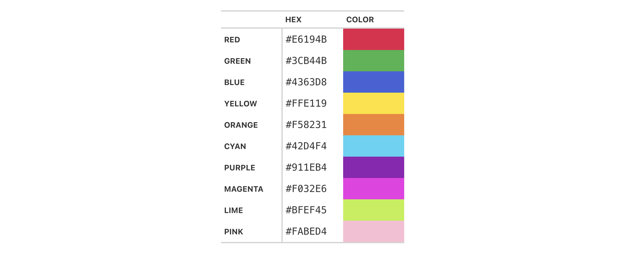
from_column() can be used to get values from a column. We'll use it in the next example, which begins with a table having a color name column and a column with the associated hexadecimal color code. To show the color in a separate column, we first create one with cols_add() (ensuring that missing values are replaced with "" via sub_missing()). Then, tab_style() is used to style that column, using color = from_column() within cell_fill().

dplyr::tibble(
  name = c(
    "red", "green", "blue", "yellow", "orange",
    "cyan", "purple", "magenta", "lime", "pink"
  ),
  hex = c(
    "#E6194B", "#3CB44B", "#4363D8", "#FFE119", "#F58231",
    "#42D4F4", "#911EB4", "#F032E6", "#BFEF45", "#FABED4"
  )
) |>
  gt(rowname_col = "name") |>
  cols_add(color = rep(NA_character_, 10)) |>
  sub_missing(missing_text = "") |>
  tab_style(
    style = cell_fill(color = from_column(column = "hex")),
    locations = cells_body(columns = color)
  ) |>
  tab_style(
    style = cell_text(font = system_fonts(name = "monospace-code")),
    locations = cells_body()
  ) |>
  opt_all_caps() |>
  cols_width(everything() ~ px(100)) |>
  tab_options(table_body.hlines.style = "none")

cell_text() also allows the use of from_column() for many ofits arguments. Let's take a small portion of data from sp500 and add an up or down arrow based on the values in the open and close columns. Within cols_add() we can create a new column (dir) with an expression to get either "red" or "green" text from a comparison of the open and close values. These values are transformed to up or down arrows with text_case_match(), using fontawesome icons in the end. However, the text values are still present and can be used by cell_text() within tab_style(). from_column() makes it possible to use the text in the cells of the dir column as color input values.

sp500 |>
  dplyr::filter(date > "2015-01-01") |>
  dplyr::slice_min(date, n = 5) |>
  dplyr::select(date, open, close) |>
  gt(rowname_col = "date") |>
  fmt_currency(columns = c(open, close)) |>
  cols_add(dir = ifelse(close < open, "red", "forestgreen")) |>
  cols_label(dir = "") |>
  text_case_match(
    "red" ~ fontawesome::fa("arrow-down"),
    "forestgreen" ~ fontawesome::fa("arrow-up")
  ) |>
  tab_style(
    style = cell_text(color = from_column("dir")),
    locations = cells_body(columns = dir)
  )

Function ID

2-10

Function Introduced

v0.2.0.5 (March 31, 2020)

See Also

cell_text(), cell_fill(), and cell_borders() as helpers for defining custom styles and cells_body() as one of many useful helper functions for targeting the locations to be styled.

Other part creation/modification functions: tab_caption(), tab_footnote(), tab_header(), tab_info(), tab_options(), tab_row_group(), tab_source_note(), tab_spanner(), tab_spanner_delim(), tab_stub_indent(), tab_stubhead(), tab_style_body()

gt documentation built on Sept. 11, 2024, 5:15 p.m.