Nothing
TensorFlow Layers
In tfestimators: Interface to 'TensorFlow' Estimators
knitr::opts_chunk$set(echo = TRUE, eval = TRUE)
The TensorFlow tf$layers module provides a high-level API that makes
it easy to construct a neural network. It provides methods that facilitate the
creation of dense (fully connected) layers and convolutional layers, adding
activation functions, and applying dropout regularization. In this tutorial,
you'll learn how to use layers to build a convolutional neural network model
to recognize the handwritten digits in the MNIST data set. The complete code
for this tutorial can be found here.
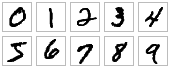
The MNIST dataset comprises 60,000
training examples and 10,000 test examples of the handwritten digits 0–9,
formatted as 28x28-pixel monochrome images.
Getting Started
Let's set up the skeleton for our TensorFlow program by adding the following code to import the necessary libraries and change the logging verbosity:
library(tensorflow)
library(tfestimators)
tf$logging$set_verbosity(tf$logging$INFO)
As you work through the tutorial, you'll add code to construct, train, and
evaluate the convolutional neural network.
Intro to Convolutional Neural Networks
Convolutional neural networks (CNNs) are the current state-of-the-art model
architecture for image classification tasks. CNNs apply a series of filters to
the raw pixel data of an image to extract and learn higher-level features, which
the model can then use for classification. CNNs contains three components:
-
Convolutional layers, which apply a specified number of convolution
filters to the image. For each subregion, the layer performs a set of
mathematical operations to produce a single value in the output feature map.
Convolutional layers then typically apply a
ReLU activation function to
the output to introduce nonlinearities into the model.
-
Pooling layers, which
downsample the image data
extracted by the convolutional layers to reduce the dimensionality of the
feature map in order to decrease processing time. A commonly used pooling
algorithm is max pooling, which extracts subregions of the feature map
(e.g., 2x2-pixel tiles), keeps their maximum value, and discards all other
values.
-
Dense (fully connected) layers, which perform classification on the
features extracted by the convolutional layers and downsampled by the
pooling layers. In a dense layer, every node in the layer is connected to
every node in the preceding layer.
Typically, a CNN is composed of a stack of convolutional modules that perform
feature extraction. Each module consists of a convolutional layer followed by a
pooling layer. The last convolutional module is followed by one or more dense
layers that perform classification. The final dense layer in a CNN contains a
single node for each target class in the model (all the possible classes the
model may predict), with a
softmax activation function to
generate a value between 0–1 for each node (the sum of all these softmax values
is equal to 1). We can interpret the softmax values for a given image as
relative measurements of how likely it is that the image falls into each target
class.
Note: For a more comprehensive walkthrough of CNN architecture, see Stanford
University's
Convolutional Neural Networks for Visual Recognition course materials.
Building the CNN MNIST Classifier {#building_the_cnn_mnist_classifier}
Let's build a model to classify the images in the MNIST dataset using the
following CNN architecture:
- Convolutional Layer #1: Applies 32 5x5 filters (extracting 5x5-pixel
subregions), with ReLU activation function
- Pooling Layer #1: Performs max pooling with a 2x2 filter and stride of 2
(which specifies that pooled regions do not overlap)
- Convolutional Layer #2: Applies 64 5x5 filters, with ReLU activation
function
- Pooling Layer #2: Again, performs max pooling with a 2x2 filter and
stride of 2
- Dense Layer #1: 1,024 neurons, with dropout regularization rate of 0.4
(probability of 0.4 that any given element will be dropped during training)
- Dense Layer #2 (Logits Layer): 10 neurons, one for each digit target
class (0–9).
The tf$layers module contains methods to create each of the three layer types
above:
conv2d(). Constructs a two-dimensional convolutional layer. Takes number
of filters, filter kernel size, padding, and activation function as
arguments.max_pooling2d(). Constructs a two-dimensional pooling layer using the
max-pooling algorithm. Takes pooling filter size and stride as arguments.dense(). Constructs a dense layer. Takes number of neurons and activation
function as arguments.
Each of these methods accepts a tensor as input and returns a transformed tensor
as output. This makes it easy to connect one layer to another: just take the
output from one layer-creation method and supply it as input to another.
The following cnn_model_fn function conforms to the interface expected by TensorFlow's Estimator API (more on this later in Create the Estimator). This example takes
MNIST feature data, labels, and mode_keys() (e.g. "train", "eval", "infer") as arguments;
configures the CNN; and returns predictions, loss, and a training operation:
cnn_model_fn <- function(features, labels, mode, params, config) {

  # Input Layer
  # Reshape X to 4-D tensor: [batch_size, width, height, channels]
  # MNIST images are 28x28 pixels, and have one color channel
  input_layer <- tf$reshape(features$x, c(-1L, 28L, 28L, 1L))

  # Convolutional Layer #1
  # Computes 32 features using a 5x5 filter with ReLU activation.
  # Padding is added to preserve width and height.
  # Input Tensor Shape: [batch_size, 28, 28, 1]
  # Output Tensor Shape: [batch_size, 28, 28, 32]
  conv1 <- tf$layers$conv2d(
    inputs = input_layer,
    filters = 32L,
    kernel_size = c(5L, 5L),
    padding = "same",
    activation = tf$nn$relu)

  # Pooling Layer #1
  # First max pooling layer with a 2x2 filter and stride of 2
  # Input Tensor Shape: [batch_size, 28, 28, 32]
  # Output Tensor Shape: [batch_size, 14, 14, 32]
  pool1 <- tf$layers$max_pooling2d(inputs = conv1, pool_size = c(2L, 2L), strides = 2L)

  # Convolutional Layer #2
  # Computes 64 features using a 5x5 filter.
  # Padding is added to preserve width and height.
  # Input Tensor Shape: [batch_size, 14, 14, 32]
  # Output Tensor Shape: [batch_size, 14, 14, 64]
  conv2 <- tf$layers$conv2d(
    inputs = pool1,
    filters = 64L,
    kernel_size = c(5L, 5L),
    padding = "same",
    activation = tf$nn$relu)

  # Pooling Layer #2
  # Second max pooling layer with a 2x2 filter and stride of 2
  # Input Tensor Shape: [batch_size, 14, 14, 64]
  # Output Tensor Shape: [batch_size, 7, 7, 64]
  pool2 <- tf$layers$max_pooling2d(inputs = conv2, pool_size = c(2L, 2L), strides = 2L)

  # Flatten tensor into a batch of vectors
  # Input Tensor Shape: [batch_size, 7, 7, 64]
  # Output Tensor Shape: [batch_size, 7 * 7 * 64]
  pool2_flat <- tf$reshape(pool2, c(-1L, 7L * 7L * 64L))

  # Dense Layer
  # Densely connected layer with 1024 neurons
  # Input Tensor Shape: [batch_size, 7 * 7 * 64]
  # Output Tensor Shape: [batch_size, 1024]
  dense <- tf$layers$dense(inputs = pool2_flat, units = 1024L, activation = tf$nn$relu)

  # Add dropout operation; 0.6 probability that element will be kept
  dropout <- tf$layers$dropout(
    inputs = dense, rate = 0.4, training = (mode == "train"))

  # Logits layer
  # Input Tensor Shape: [batch_size, 1024]
  # Output Tensor Shape: [batch_size, 10]
  logits <- tf$layers$dense(inputs = dropout, units = 10L)

  # Generate Predictions (for prediction mode)
  predicted_classes <- tf$argmax(input = logits, axis = 1L, name = "predicted_classes")
  if (mode == "infer") {
    predictions <- list(
      classes = predicted_classes,
      probabilities = tf$nn$softmax(logits, name = "softmax_tensor")
    )
    return(estimator_spec(mode = mode, predictions = predictions))
  }

  # Calculate Loss (for both "train" and "eval" modes)
  onehot_labels <- tf$one_hot(indices = tf$cast(labels, tf$int32), depth = 10L)
  loss <- tf$losses$softmax_cross_entropy(
    onehot_labels = onehot_labels, logits = logits)

  # Configure the Training Op (for "train" mode)
  if (mode == "train") {
    optimizer <- tf$train$GradientDescentOptimizer(learning_rate = 0.001)
    train_op <- optimizer$minimize(
      loss = loss,
      global_step = tf$train$get_global_step())
    return(estimator_spec(mode = mode, loss = loss, train_op = train_op))
  }

  # Add evaluation metrics (for EVAL mode)
  eval_metric_ops <- list(accuracy = tf$metrics$accuracy(
    labels = labels, predictions = predicted_classes))

  return(estimator_spec(
    mode = mode, loss = loss, eval_metric_ops = eval_metric_ops))
}
The following sections (with headings corresponding to each code block above)
dive deeper into the tf$layers code used to create each layer, as well as how
to calculate loss, configure the training op, and generate predictions. If
you're already experienced with CNNs and creatings estimators in tfestimators,
and find the above code intuitive, you may want to skim these sections or just
skip ahead to "Training and Evaluating the CNN MNIST
Classifier".
Input Layer
The methods in the layers module for creating convolutional and pooling layers
for two-dimensional image data expect input tensors to have a shape of
[batch_size, image_width, image_height,
channels]
, defined as follows:
batch_size. Size of the subset of examples to use when performing
gradient descent during training.image_width. Width of the example images.image_height. Height of the example images.channels. Number of color channels in the example images. For color
images, the number of channels is 3 (red, green, blue). For monochrome
images, there is just 1 channel (black).
Here, our MNIST dataset is composed of monochrome 28x28 pixel images, so the
desired shape for our input layer is [batch_size, 28, 28,
1].
To convert our input feature map (features) to this shape, we can perform the
following reshape operation:
input_layer <- tf$reshape(features$x, c(-1L, 28L, 28L, 1L))
Note that we've indicated -1 for batch size, which specifies that this
dimension should be dynamically computed based on the number of input values in
features$x, holding the size of all other dimensions constant. This allows
us to treat batch_size as a hyperparameter that we can tune. For example, if
we feed examples into our model in batches of 5, features$x will contain
3,920 values (one value for each pixel in each image), and input_layer will
have a shape of [5, 28, 28, 1]. Similarly, if we feed examples in batches of
100, features$x will contain 78,400 values, and input_layer will have a
shape of [100, 28, 28, 1].
Convolutional Layer #1
In our first convolutional layer, we want to apply 32 5x5 filters to the input
layer, with a ReLU activation function. We can use the conv2d() method in the
layers module to create this layer as follows:
conv1 <- tf$layers$conv2d(
    inputs = input_layer,
    filters = 32L,
    kernel_size = c(5L, 5L),
    padding = "same",
    activation = tf$nn$relu)
The inputs argument specifies our input tensor, which must have the shape
[batch_size, image_width, image_height,
channels]
. Here, we're connecting our first convolutional layer
to input_layer, which has the shape [batch_size, 28, 28,
1].
Note: conv2d() will instead accept a shape of
[channels, batch_size, image_width,
image_height]
when passed the argument
data_format=channels_first.
The filters argument specifies the number of filters to apply (here, 32), and
kernel_size specifies the dimensions of the filters as [width,
height] (here, [5, 5]).
TIP: If filter width and height have the same value, you can instead specify a
single integer for kernel_size—e.g., kernel_size=5.
The padding argument specifies one of two enumerated values
(case-insensitive): valid (default value) or same. To specify that the
output tensor should have the same width and height values as the input tensor,
we set padding=same here, which instructs TensorFlow to add 0 values to the
edges of the output tensor to preserve width and height of 28. (Without padding,
a 5x5 convolution over a 28x28 tensor will produce a 24x24 tensor, as there are
24x24 locations to extract a 5x5 tile from a 28x28 grid.)
The activation argument specifies the activation function to apply to the
output of the convolution. Here, we specify ReLU activation with
@{tf.nn.relu}.
Our output tensor produced by conv2d() has a shape of
[batch_size, 28, 28, 32]: the same width and height
dimensions as the input, but now with 32 channels holding the output from each
of the filters.
Pooling Layer #1
Next, we connect our first pooling layer to the convolutional layer we just
created. We can use the max_pooling2d() method in layers to construct a
layer that performs max pooling with a 2x2 filter and stride of 2:
pool1 <- tf$layers$max_pooling2d(inputs = conv1, pool_size = c(2L, 2L), strides = 2L)
Again, inputs specifies the input tensor, with a shape of
[batch_size, image_width, image_height,
channels]. Here, our input tensor is conv1, the output from
the first convolutional layer, which has a shape of [batch_size,
28, 28, 32].
Note: As with conv2d(), max_pooling2d() will instead
accept a shape of [channels, batch_size,
image_width, image_height] when passed the argument
data_format=channels_first.
The pool_size argument specifies the size of the max pooling filter as
[width,
height]
(here, [2, 2]). If both
dimensions have the same value, you can instead specify a single integer (e.g.,
pool_size = 2).
The strides argument specifies the size of the stride. Here, we set a stride
of 2, which indicates that the subregions extracted by the filter should be
separated by 2 pixels in both the width and height dimensions (for a 2x2 filter,
this means that none of the regions extracted will overlap). If you want to set
different stride values for width and height, you can instead specify a tuple or
list (e.g., stride = c(3, 6)).
Our output tensor produced by max_pooling2d() (pool1) has a shape of
[batch_size, 14, 14, 32]: the 2x2 filter reduces width and
height by 50% each.
Convolutional Layer #2 and Pooling Layer #2
We can connect a second convolutional and pooling layer to our CNN using
conv2d() and max_pooling2d() as before. For convolutional layer #2, we
configure 64 5x5 filters with ReLU activation, and for pooling layer #2, we use
the same specs as pooling layer #1 (a 2x2 max pooling filter with stride of 2):
conv2 <- tf$layers$conv2d(
inputs = pool1,
filters = 64L,
kernel_size = c(5L, 5L),
padding = "same",
activation = tf$nn$relu)
pool2 <- tf$layers$max_pooling2d(inputs = conv2, pool_size = c(2L, 2L), strides = 2L)
Note that convolutional layer #2 takes the output tensor of our first pooling
layer (pool1) as input, and produces the tensor conv2 as output. conv2
has a shape of [batch_size, 14, 14, 64], the same width
and height as pool1 (due to padding="same"), and 64 channels for the 64
filters applied.
Pooling layer #2 takes conv2 as input, producing pool2 as output. pool2
has shape [batch_size, 7, 7, 64] (50% reduction of width
and height from conv2).
Dense Layer
Next, we want to add a dense layer (with 1,024 neurons and ReLU activation) to
our CNN to perform classification on the features extracted by the
convolution/pooling layers. Before we connect the layer, however, we'll flatten
our feature map (pool2) to shape [batch_size,
features], so that our tensor has only two dimensions:
pool2_flat <- tf$reshape(pool2, c(-1L, 7L * 7L * 64L))
In the reshape() operation above, the -1 signifies that the batch_size
dimension will be dynamically calculated based on the number of examples in our
input data. Each example has 7 (pool2 width) * 7 (pool2 height) * 64
(pool2 channels) features, so we want the features dimension to have a value
of 7 * 7 * 64 (3136 in total). The output tensor, pool2_flat, has shape
[batch_size, 3136].
Now, we can use the dense() method in layers to connect our dense layer as
follows:
dense <- tf$layers$dense(inputs = pool2_flat, units = 1024L, activation = tf$nn$relu)
The inputs argument specifies the input tensor: our flattened feature map,
pool2_flat. The units argument specifies the number of neurons in the dense
layer (1,024). The activation argument takes the activation function; again,
we'll use tf.nn.relu to add ReLU activation.
To help improve the results of our model, we also apply dropout regularization
to our dense layer, using the dropout method in layers:
dropout <- tf$layers$dropout(
inputs = dense, rate = 0.4, training = (mode == "train"))
Again, inputs specifies the input tensor, which is the output tensor from our
dense layer (dense).
The rate argument specifies the dropout rate; here, we use 0.4, which means
40% of the elements will be randomly dropped out during training.
The training argument takes a boolean specifying whether or not the model is
currently being run in training mode; dropout will only be performed if
training is True. Here, we check if the mode passed to our model function
cnn_model_fn is "train mode.
Our output tensor dropout has shape [batch_size, 1024].
Logits Layer
The final layer in our neural network is the logits layer, which will return the
raw values for our predictions. We create a dense layer with 10 neurons (one for
each target class 0–9), with linear activation (the default):
logits <- tf$layers$dense(inputs = dropout, units = 10L)
Our final output tensor of the CNN, logits, has shape
[batch_size, 10].
Generate Predictions {#generate_predictions}
The logits layer of our model returns our predictions as raw values in a
[batch_size, 10]-dimensional tensor. Let's convert these
raw values into two different formats that our model function can return:
- The predicted class for each example: a digit from 0–9.
- The probabilities for each possible target class for each example: the
probability that the example is a 0, is a 1, is a 2, etc.
For a given example, our predicted class is the element in the corresponding row
of the logits tensor with the highest raw value. We can find the index of this
element using the @{tf.argmax}
function:
tf$argmax(input = logits, axis = 1L)
The input argument specifies the tensor from which to extract maximum
values—here logits. The axis argument specifies the axis of the input
tensor along which to find the greatest value. Here, we want to find the largest
value along the dimension with index of 1, which corresponds to our predictions
(recall that our logits tensor has shape [batch_size,
10]).
We can derive probabilities from our logits layer by applying softmax activation
using @{tf.nn.softmax}:
tf$nn$softmax(logits, name = "softmax_tensor")
Note: We use the name argument to explicitly name this operation
softmax_tensor, so we can reference it later.
We compile our predictions in a dict, and return an estimator_spec object:
predicted_classes <- tf$argmax(input = logits, axis = 1L)
if (mode == "infer") {
predictions <- list(
classes = predicted_classes,
probabilities = tf$nn$softmax(logits, name = "softmax_tensor")
)
return(estimator_spec(mode = mode, predictions = predictions))
}
Calculate Loss {#calculating-loss}
For both training and evaluation, we need to define a
loss function
that measures how closely the model's predictions match the target classes. For
multiclass classification problems like MNIST,
cross entropy is typically used
as the loss metric. The following code calculates cross entropy when the model
runs in either TRAIN or EVAL mode:
onehot_labels <- tf$one_hot(indices = tf$cast(labels, tf$int32), depth = 10L)
loss <- tf$losses$softmax_cross_entropy(
onehot_labels = onehot_labels, logits = logits)
Let's take a closer look at what's happening above.
Our labels tensor contains a list of predictions for our examples, e.g. [1,
9, ...]. In order to calculate cross-entropy, first we need to convert labels
to the corresponding
one-hot encoding (quora.com/What-is-one-hot-encoding-and-when-is-it-used-in-data-science):
[[0, 1, 0, 0, 0, 0, 0, 0, 0, 0],
[0, 0, 0, 0, 0, 0, 0, 0, 0, 1],
...]
We use the tf$one_hot function
to perform this conversion. tf$one_hot has two required arguments:
indices. The locations in the one-hot tensor that will have "on
values"—i.e., the locations of 1 values in the tensor shown above.depth. The depth of the one-hot tensor—i.e., the number of target classes.
Here, the depth is 10.
The following code creates the one-hot tensor for our labels, onehot_labels:
onehot_labels <- tf$one_hot(indices = tf$cast(labels, tf$int32), depth = 10L)
Because labels contains a series of values from 0–9, indices is just our
labels tensor, with values cast to integers. The depth is 10 because we
have 10 possible target classes, one for each digit.
Next, we compute cross-entropy of onehot_labels and the softmax of the
predictions from our logits layer. tf$losses$softmax_cross_entropy() takes
onehot_labels and logits as arguments, performs softmax activation on
logits, calculates cross-entropy, and returns our loss as a scalar Tensor:
loss <- tf$losses$softmax_cross_entropy(
onehot_labels = onehot_labels, logits = logits)
Configure the Training Op
In the previous section, we defined loss for our CNN as the softmax
cross-entropy of the logits layer and our labels. Let's configure our model to
optimize this loss value during training. We'll use a learning rate of 0.001 and
stochastic gradient descent
as the optimization algorithm:
if (mode == "train") {
optimizer <- tf$train$GradientDescentOptimizer(learning_rate = 0.001)
train_op <- optimizer$minimize(
loss = loss,
global_step = tf$train$get_global_step())
return(estimator_spec(mode = mode, loss = loss, train_op = train_op))
}
Add evaluation metrics
To add accuracy metric in our model, we define eval_metric_ops dict in EVAL
mode as follows:
eval_metric_ops <- list(accuracy = tf$metrics$accuracy(
labels = labels, predictions = predicted_classes))
return(estimator_spec(
mode = mode, loss = loss, eval_metric_ops = eval_metric_ops))
Training and Evaluating the CNN MNIST Classifier {#training_and_evaluating_the_cnn_mnist_classifier}
We've coded our MNIST CNN model function; now we're ready to train and evaluate
it.
Load Training and Test Data
First, let's load our training and test data:
np <- import("numpy", convert = FALSE)
# Load training and eval data
mnist <- tf$contrib$learn$datasets$load_dataset("mnist")
train_data <- np$asmatrix(mnist$train$images, dtype = np$float32)
train_labels <- np$asarray(mnist$train$labels, dtype = np$int32)
eval_data <- np$asmatrix(mnist$test$images, dtype = np$float32)
eval_labels <- np$asarray(mnist$test$labels, dtype = np$int32)
We store the training feature data (the raw pixel values for 55,000 images of
hand-drawn digits) and training labels (the corresponding value from 0–9 for
each image) as numpy
arrays
in train_data and train_labels, respectively. Similarly, we store the
evaluation feature data (10,000 images) and evaluation labels in eval_data
and eval_labels, respectively.
Create the Estimator {#create-the-estimator}
Next, let's create an estimator (a TensorFlow class for performing high-level
model training, evaluation, and inference) for our model.
# Create the Estimator
mnist_classifier <- estimator(
model_fn = cnn_model_fn, model_dir = "/tmp/mnist_convnet_model")
The model_fn argument specifies the model function to use for training,
evaluation, and prediction; we pass it the cnn_model_fn we created in
"Building the CNN MNIST Classifier." The
model_dir argument specifies the directory where model data (checkpoints) will
be saved (here, we specify the temp directory /tmp/mnist_convnet_model, but
feel free to change to another directory of your choice).
Note: For an in-depth walkthrough of the TensorFlow Estimator API, see the
tutorial for custom estimator.
Set Up a Logging Hook {#set_up_a_logging_hook}
Since CNNs can take a while to train, let's set up some logging so we can track
progress during training. We can use TensorFlow's SessionRunHook to create a
hook_logging_tensor that will log the predicted classes from the argmax operation.
# Set up logging for predicted classes
tensors_to_log <- list(predicted_classes = "predicted_classes")
logging_hook <- hook_logging_tensor(
tensors = tensors_to_log, every_n_iter = 50)
We store a dict of the tensors we want to log in tensors_to_log. Each key is a
label of our choice that will be printed in the log output, and the
corresponding label is the name of a Tensor in the TensorFlow graph. Here, our
predicted classes can be found in predicted_classes, the name we gave our argmax
operation earlier when we generated the predicted classes in cnn_model_fn.
Next, we create the hook_logging_tensor, passing tensors_to_log to the
tensors argument. We set every_n_iter = 50, which specifies that probabilities
should be logged after every 50 steps of training.
Train the Model
Now we're ready to train our model, which we can do by creating train_input_fn
ans calling train() on mnist_classifier.
# Train the model
train_input_fn <- function(features_as_named_list) {
tf$estimator$inputs$numpy_input_fn(
x = list(x = train_data),
y = train_labels,
batch_size = 100L,
num_epochs = NULL,
shuffle = TRUE)
}
train(
mnist_classifier,
input_fn = train_input_fn,
steps = 20,
hooks = logging_hook)
In the numpy_input_fn call, we pass the training feature data and labels to
x (as a dict) and y, respectively. We set a batch_size of 100 (which
means that the model will train on minibatches of 100 examples at each step).
num_epochs = NULL means that the model will train until the specified number of
steps is reached. We also set shuffle = TRUE to shuffle the training data.
In the train call, we set steps = 2
(which means the model will train for 10 steps total).
Evaluate the Model
Once training is complete, we want to evaluate our model to determine its
accuracy on the MNIST test set. We call the evaluate method, which evaluates
the metrics we specified in eval_metric_ops argument in the model_fn.
# Evaluate the model and print results
eval_input_fn <- function(features_as_named_list) {
tf$estimator$inputs$numpy_input_fn(
x = list(x = eval_data),
y = eval_labels,
batch_size = 100L,
num_epochs = NULL,
shuffle = TRUE)
}
evaluate(
mnist_classifier,
input_fn = eval_input_fn,
steps = 10,
hooks = logging_hook)
To create eval_input_fn, we set num_epochs = 1, so that the model evaluates
the metrics over one epoch of data and returns the result. We also set
shuffle = FALSE to iterate through the data sequentially.
We pass our logging_hook to the hooks argument, so that it will be triggered during
evaluation.
Run the Model
We've coded the CNN model function, Estimator, and the training/evaluation
logic; now let's see the results.
As the model trains, you'll see log output like the following:
INFO:tensorflow:Create CheckpointSaverHook.
INFO:tensorflow:Restoring parameters from /tmp/mnist_convnet_model/model.ckpt-5
INFO:tensorflow:Saving checkpoints for 6 into /tmp/mnist_convnet_model/model.ckpt.
INFO:tensorflow:loss = 2.29727, step = 6
INFO:tensorflow:Saving checkpoints for 7 into /tmp/mnist_convnet_model/model.ckpt.
INFO:tensorflow:Loss for final step: 2.30916.
You'll see log output like the following during model evaluation with the predicted_classes that we included in the logging_hook:
INFO:tensorflow:Starting evaluation at 2017-07-04-17:05:28
INFO:tensorflow:Restoring parameters from /tmp/mnist_convnet_model/model.ckpt-19
INFO:tensorflow:predicted_classes = [6 9 1 9 9 1 9 1 9 6 1 9 9 9 9 1 9 9 9 3 1 1 1 9 6 1 9 9 9 9 9 9 1 1 9 9 9
9 9 9 9 1 9 9 1 4 4 1 9 1 9 9 1 9 9 9 9 9 9 1 6 9 9 1 9 6 9 9 9 9 9 9 1 9
9 3 9 9 9 9 1 9 9 9 3 9 1 9 9 9 9 9 9 9 9 9 1 9 9 9]
INFO:tensorflow:Evaluation [1/10]
INFO:tensorflow:Evaluation [2/10]
INFO:tensorflow:predicted_classes = [9 9 1 9 1 9 9 9 9 9 9 9 9 9 9 9 9 9 1 4 1 9 9 9 1 9 9 9 9 9 1 9 4 9 1 1 9
9 1 1 9 9 1 9 9 9 9 1 9 9 9 9 4 9 9 9 9 4 9 9 9 9 9 9 9 9 9 9 9 9 9 9 9 9
9 1 9 9 9 9 9 9 9 9 1 1 9 9 9 9 1 9 9 9 9 9 9 9 9 9] (0.204 sec)
INFO:tensorflow:Evaluation [3/10]
INFO:tensorflow:Evaluation [4/10]
...
Try the tfestimators package in your browser
Any scripts or data that you put into this service are public.
tfestimators documentation built on Aug. 19, 2025, 1:15 a.m.
R Package Documentation
Browse R Packages
We want your feedback!
Note that we can't provide technical support on individual packages. You should contact the package authors for that.
knitr::opts_chunk$set(echo = TRUE, eval = TRUE)
The TensorFlow tf$layers module provides a high-level API that makes
it easy to construct a neural network. It provides methods that facilitate the
creation of dense (fully connected) layers and convolutional layers, adding
activation functions, and applying dropout regularization. In this tutorial,
you'll learn how to use layers to build a convolutional neural network model
to recognize the handwritten digits in the MNIST data set. The complete code
for this tutorial can be found here.
The MNIST dataset comprises 60,000 training examples and 10,000 test examples of the handwritten digits 0–9, formatted as 28x28-pixel monochrome images.
Getting Started
Let's set up the skeleton for our TensorFlow program by adding the following code to import the necessary libraries and change the logging verbosity:
library(tensorflow) library(tfestimators) tf$logging$set_verbosity(tf$logging$INFO)
As you work through the tutorial, you'll add code to construct, train, and evaluate the convolutional neural network.
Intro to Convolutional Neural Networks
Convolutional neural networks (CNNs) are the current state-of-the-art model architecture for image classification tasks. CNNs apply a series of filters to the raw pixel data of an image to extract and learn higher-level features, which the model can then use for classification. CNNs contains three components:
-
Convolutional layers, which apply a specified number of convolution filters to the image. For each subregion, the layer performs a set of mathematical operations to produce a single value in the output feature map. Convolutional layers then typically apply a ReLU activation function to the output to introduce nonlinearities into the model.
-
Pooling layers, which downsample the image data extracted by the convolutional layers to reduce the dimensionality of the feature map in order to decrease processing time. A commonly used pooling algorithm is max pooling, which extracts subregions of the feature map (e.g., 2x2-pixel tiles), keeps their maximum value, and discards all other values.
-
Dense (fully connected) layers, which perform classification on the features extracted by the convolutional layers and downsampled by the pooling layers. In a dense layer, every node in the layer is connected to every node in the preceding layer.
Typically, a CNN is composed of a stack of convolutional modules that perform feature extraction. Each module consists of a convolutional layer followed by a pooling layer. The last convolutional module is followed by one or more dense layers that perform classification. The final dense layer in a CNN contains a single node for each target class in the model (all the possible classes the model may predict), with a softmax activation function to generate a value between 0–1 for each node (the sum of all these softmax values is equal to 1). We can interpret the softmax values for a given image as relative measurements of how likely it is that the image falls into each target class.
Note: For a more comprehensive walkthrough of CNN architecture, see Stanford University's Convolutional Neural Networks for Visual Recognition course materials.
Building the CNN MNIST Classifier {#building_the_cnn_mnist_classifier}
Let's build a model to classify the images in the MNIST dataset using the following CNN architecture:
- Convolutional Layer #1: Applies 32 5x5 filters (extracting 5x5-pixel subregions), with ReLU activation function
- Pooling Layer #1: Performs max pooling with a 2x2 filter and stride of 2 (which specifies that pooled regions do not overlap)
- Convolutional Layer #2: Applies 64 5x5 filters, with ReLU activation function
- Pooling Layer #2: Again, performs max pooling with a 2x2 filter and stride of 2
- Dense Layer #1: 1,024 neurons, with dropout regularization rate of 0.4 (probability of 0.4 that any given element will be dropped during training)
- Dense Layer #2 (Logits Layer): 10 neurons, one for each digit target class (0–9).
The tf$layers module contains methods to create each of the three layer types
above:
conv2d(). Constructs a two-dimensional convolutional layer. Takes number of filters, filter kernel size, padding, and activation function as arguments.max_pooling2d(). Constructs a two-dimensional pooling layer using the max-pooling algorithm. Takes pooling filter size and stride as arguments.dense(). Constructs a dense layer. Takes number of neurons and activation function as arguments.
Each of these methods accepts a tensor as input and returns a transformed tensor as output. This makes it easy to connect one layer to another: just take the output from one layer-creation method and supply it as input to another.
The following cnn_model_fn function conforms to the interface expected by TensorFlow's Estimator API (more on this later in Create the Estimator). This example takes
MNIST feature data, labels, and mode_keys() (e.g. "train", "eval", "infer") as arguments;
configures the CNN; and returns predictions, loss, and a training operation:
cnn_model_fn <- function(features, labels, mode, params, config) { # Input Layer # Reshape X to 4-D tensor: [batch_size, width, height, channels] # MNIST images are 28x28 pixels, and have one color channel input_layer <- tf$reshape(features$x, c(-1L, 28L, 28L, 1L)) # Convolutional Layer #1 # Computes 32 features using a 5x5 filter with ReLU activation. # Padding is added to preserve width and height. # Input Tensor Shape: [batch_size, 28, 28, 1] # Output Tensor Shape: [batch_size, 28, 28, 32] conv1 <- tf$layers$conv2d( inputs = input_layer, filters = 32L, kernel_size = c(5L, 5L), padding = "same", activation = tf$nn$relu) # Pooling Layer #1 # First max pooling layer with a 2x2 filter and stride of 2 # Input Tensor Shape: [batch_size, 28, 28, 32] # Output Tensor Shape: [batch_size, 14, 14, 32] pool1 <- tf$layers$max_pooling2d(inputs = conv1, pool_size = c(2L, 2L), strides = 2L) # Convolutional Layer #2 # Computes 64 features using a 5x5 filter. # Padding is added to preserve width and height. # Input Tensor Shape: [batch_size, 14, 14, 32] # Output Tensor Shape: [batch_size, 14, 14, 64] conv2 <- tf$layers$conv2d( inputs = pool1, filters = 64L, kernel_size = c(5L, 5L), padding = "same", activation = tf$nn$relu) # Pooling Layer #2 # Second max pooling layer with a 2x2 filter and stride of 2 # Input Tensor Shape: [batch_size, 14, 14, 64] # Output Tensor Shape: [batch_size, 7, 7, 64] pool2 <- tf$layers$max_pooling2d(inputs = conv2, pool_size = c(2L, 2L), strides = 2L) # Flatten tensor into a batch of vectors # Input Tensor Shape: [batch_size, 7, 7, 64] # Output Tensor Shape: [batch_size, 7 * 7 * 64] pool2_flat <- tf$reshape(pool2, c(-1L, 7L * 7L * 64L)) # Dense Layer # Densely connected layer with 1024 neurons # Input Tensor Shape: [batch_size, 7 * 7 * 64] # Output Tensor Shape: [batch_size, 1024] dense <- tf$layers$dense(inputs = pool2_flat, units = 1024L, activation = tf$nn$relu) # Add dropout operation; 0.6 probability that element will be kept dropout <- tf$layers$dropout( inputs = dense, rate = 0.4, training = (mode == "train")) # Logits layer # Input Tensor Shape: [batch_size, 1024] # Output Tensor Shape: [batch_size, 10] logits <- tf$layers$dense(inputs = dropout, units = 10L) # Generate Predictions (for prediction mode) predicted_classes <- tf$argmax(input = logits, axis = 1L, name = "predicted_classes") if (mode == "infer") { predictions <- list( classes = predicted_classes, probabilities = tf$nn$softmax(logits, name = "softmax_tensor") ) return(estimator_spec(mode = mode, predictions = predictions)) } # Calculate Loss (for both "train" and "eval" modes) onehot_labels <- tf$one_hot(indices = tf$cast(labels, tf$int32), depth = 10L) loss <- tf$losses$softmax_cross_entropy( onehot_labels = onehot_labels, logits = logits) # Configure the Training Op (for "train" mode) if (mode == "train") { optimizer <- tf$train$GradientDescentOptimizer(learning_rate = 0.001) train_op <- optimizer$minimize( loss = loss, global_step = tf$train$get_global_step()) return(estimator_spec(mode = mode, loss = loss, train_op = train_op)) } # Add evaluation metrics (for EVAL mode) eval_metric_ops <- list(accuracy = tf$metrics$accuracy( labels = labels, predictions = predicted_classes)) return(estimator_spec( mode = mode, loss = loss, eval_metric_ops = eval_metric_ops)) }
The following sections (with headings corresponding to each code block above)
dive deeper into the tf$layers code used to create each layer, as well as how
to calculate loss, configure the training op, and generate predictions. If
you're already experienced with CNNs and creatings estimators in tfestimators,
and find the above code intuitive, you may want to skim these sections or just
skip ahead to "Training and Evaluating the CNN MNIST
Classifier".
Input Layer
The methods in the layers module for creating convolutional and pooling layers
for two-dimensional image data expect input tensors to have a shape of
[batch_size, image_width, image_height,
channels], defined as follows:
batch_size. Size of the subset of examples to use when performing gradient descent during training.image_width. Width of the example images.image_height. Height of the example images.channels. Number of color channels in the example images. For color images, the number of channels is 3 (red, green, blue). For monochrome images, there is just 1 channel (black).
Here, our MNIST dataset is composed of monochrome 28x28 pixel images, so the
desired shape for our input layer is [batch_size, 28, 28,
1].
To convert our input feature map (features) to this shape, we can perform the
following reshape operation:
input_layer <- tf$reshape(features$x, c(-1L, 28L, 28L, 1L))
Note that we've indicated -1 for batch size, which specifies that this
dimension should be dynamically computed based on the number of input values in
features$x, holding the size of all other dimensions constant. This allows
us to treat batch_size as a hyperparameter that we can tune. For example, if
we feed examples into our model in batches of 5, features$x will contain
3,920 values (one value for each pixel in each image), and input_layer will
have a shape of [5, 28, 28, 1]. Similarly, if we feed examples in batches of
100, features$x will contain 78,400 values, and input_layer will have a
shape of [100, 28, 28, 1].
Convolutional Layer #1
In our first convolutional layer, we want to apply 32 5x5 filters to the input
layer, with a ReLU activation function. We can use the conv2d() method in the
layers module to create this layer as follows:
conv1 <- tf$layers$conv2d( inputs = input_layer, filters = 32L, kernel_size = c(5L, 5L), padding = "same", activation = tf$nn$relu)
The inputs argument specifies our input tensor, which must have the shape
[batch_size, image_width, image_height,
channels]. Here, we're connecting our first convolutional layer
to input_layer, which has the shape [batch_size, 28, 28,
1].
Note:
conv2d()will instead accept a shape of[channels, batch_size, image_width, image_height]when passed the argumentdata_format=channels_first.
The filters argument specifies the number of filters to apply (here, 32), and
kernel_size specifies the dimensions of the filters as [width,
height] (here, [5, 5]).
TIP: If filter width and height have the same value, you can instead specify a
single integer for kernel_size—e.g., kernel_size=5.
The padding argument specifies one of two enumerated values
(case-insensitive): valid (default value) or same. To specify that the
output tensor should have the same width and height values as the input tensor,
we set padding=same here, which instructs TensorFlow to add 0 values to the
edges of the output tensor to preserve width and height of 28. (Without padding,
a 5x5 convolution over a 28x28 tensor will produce a 24x24 tensor, as there are
24x24 locations to extract a 5x5 tile from a 28x28 grid.)
The activation argument specifies the activation function to apply to the
output of the convolution. Here, we specify ReLU activation with
@{tf.nn.relu}.
Our output tensor produced by conv2d() has a shape of
[batch_size, 28, 28, 32]: the same width and height
dimensions as the input, but now with 32 channels holding the output from each
of the filters.
Pooling Layer #1
Next, we connect our first pooling layer to the convolutional layer we just
created. We can use the max_pooling2d() method in layers to construct a
layer that performs max pooling with a 2x2 filter and stride of 2:
pool1 <- tf$layers$max_pooling2d(inputs = conv1, pool_size = c(2L, 2L), strides = 2L)
Again, inputs specifies the input tensor, with a shape of
[batch_size, image_width, image_height,
channels]. Here, our input tensor is conv1, the output from
the first convolutional layer, which has a shape of [batch_size,
28, 28, 32].
Note: As with
conv2d(),max_pooling2d()will instead accept a shape of[channels, batch_size, image_width, image_height]when passed the argumentdata_format=channels_first.
The pool_size argument specifies the size of the max pooling filter as
[width, height] (here, [2, 2]). If both
dimensions have the same value, you can instead specify a single integer (e.g.,
pool_size = 2).
The strides argument specifies the size of the stride. Here, we set a stride
of 2, which indicates that the subregions extracted by the filter should be
separated by 2 pixels in both the width and height dimensions (for a 2x2 filter,
this means that none of the regions extracted will overlap). If you want to set
different stride values for width and height, you can instead specify a tuple or
list (e.g., stride = c(3, 6)).
Our output tensor produced by max_pooling2d() (pool1) has a shape of
[batch_size, 14, 14, 32]: the 2x2 filter reduces width and
height by 50% each.
Convolutional Layer #2 and Pooling Layer #2
We can connect a second convolutional and pooling layer to our CNN using
conv2d() and max_pooling2d() as before. For convolutional layer #2, we
configure 64 5x5 filters with ReLU activation, and for pooling layer #2, we use
the same specs as pooling layer #1 (a 2x2 max pooling filter with stride of 2):
conv2 <- tf$layers$conv2d(
    inputs = pool1,
    filters = 64L,
    kernel_size = c(5L, 5L),
    padding = "same",
    activation = tf$nn$relu)

pool2 <- tf$layers$max_pooling2d(inputs = conv2, pool_size = c(2L, 2L), strides = 2L)
Note that convolutional layer #2 takes the output tensor of our first pooling
layer (pool1) as input, and produces the tensor conv2 as output. conv2
has a shape of [batch_size, 14, 14, 64], the same width
and height as pool1 (due to padding="same"), and 64 channels for the 64
filters applied.
Pooling layer #2 takes conv2 as input, producing pool2 as output. pool2
has shape [batch_size, 7, 7, 64] (50% reduction of width
and height from conv2).
Dense Layer
Next, we want to add a dense layer (with 1,024 neurons and ReLU activation) to
our CNN to perform classification on the features extracted by the
convolution/pooling layers. Before we connect the layer, however, we'll flatten
our feature map (pool2) to shape [batch_size,
features], so that our tensor has only two dimensions:
pool2_flat <- tf$reshape(pool2, c(-1L, 7L * 7L * 64L))
In the reshape() operation above, the -1 signifies that the batch_size
dimension will be dynamically calculated based on the number of examples in our
input data. Each example has 7 (pool2 width) * 7 (pool2 height) * 64
(pool2 channels) features, so we want the features dimension to have a value
of 7 * 7 * 64 (3136 in total). The output tensor, pool2_flat, has shape
[batch_size, 3136].
Now, we can use the dense() method in layers to connect our dense layer as
follows:
dense <- tf$layers$dense(inputs = pool2_flat, units = 1024L, activation = tf$nn$relu)
The inputs argument specifies the input tensor: our flattened feature map,
pool2_flat. The units argument specifies the number of neurons in the dense
layer (1,024). The activation argument takes the activation function; again,
we'll use tf.nn.relu to add ReLU activation.
To help improve the results of our model, we also apply dropout regularization
to our dense layer, using the dropout method in layers:
dropout <- tf$layers$dropout(
    inputs = dense, rate = 0.4, training = (mode == "train"))
Again, inputs specifies the input tensor, which is the output tensor from our
dense layer (dense).
The rate argument specifies the dropout rate; here, we use 0.4, which means
40% of the elements will be randomly dropped out during training.
The training argument takes a boolean specifying whether or not the model is
currently being run in training mode; dropout will only be performed if
training is True. Here, we check if the mode passed to our model function
cnn_model_fn is "train mode.
Our output tensor dropout has shape [batch_size, 1024].
Logits Layer
The final layer in our neural network is the logits layer, which will return the raw values for our predictions. We create a dense layer with 10 neurons (one for each target class 0–9), with linear activation (the default):
logits <- tf$layers$dense(inputs = dropout, units = 10L)
Our final output tensor of the CNN, logits, has shape
[batch_size, 10].
Generate Predictions {#generate_predictions}
The logits layer of our model returns our predictions as raw values in a
[batch_size, 10]-dimensional tensor. Let's convert these
raw values into two different formats that our model function can return:
- The predicted class for each example: a digit from 0–9.
- The probabilities for each possible target class for each example: the probability that the example is a 0, is a 1, is a 2, etc.
For a given example, our predicted class is the element in the corresponding row of the logits tensor with the highest raw value. We can find the index of this element using the @{tf.argmax} function:
tf$argmax(input = logits, axis = 1L)
The input argument specifies the tensor from which to extract maximum
values—here logits. The axis argument specifies the axis of the input
tensor along which to find the greatest value. Here, we want to find the largest
value along the dimension with index of 1, which corresponds to our predictions
(recall that our logits tensor has shape [batch_size,
10]).
We can derive probabilities from our logits layer by applying softmax activation using @{tf.nn.softmax}:
tf$nn$softmax(logits, name = "softmax_tensor")
Note: We use the
nameargument to explicitly name this operationsoftmax_tensor, so we can reference it later.
We compile our predictions in a dict, and return an estimator_spec object:
predicted_classes <- tf$argmax(input = logits, axis = 1L)
if (mode == "infer") {
  predictions <- list(
    classes = predicted_classes,
    probabilities = tf$nn$softmax(logits, name = "softmax_tensor")
  )
  return(estimator_spec(mode = mode, predictions = predictions))
}
Calculate Loss {#calculating-loss}
For both training and evaluation, we need to define a
loss function
that measures how closely the model's predictions match the target classes. For
multiclass classification problems like MNIST,
cross entropy is typically used
as the loss metric. The following code calculates cross entropy when the model
runs in either TRAIN or EVAL mode:
onehot_labels <- tf$one_hot(indices = tf$cast(labels, tf$int32), depth = 10L)
loss <- tf$losses$softmax_cross_entropy(
  onehot_labels = onehot_labels, logits = logits)
Let's take a closer look at what's happening above.
Our labels tensor contains a list of predictions for our examples, e.g. [1,
9, ...]. In order to calculate cross-entropy, first we need to convert labels
to the corresponding
one-hot encoding (quora.com/What-is-one-hot-encoding-and-when-is-it-used-in-data-science):
[[0, 1, 0, 0, 0, 0, 0, 0, 0, 0],
 [0, 0, 0, 0, 0, 0, 0, 0, 0, 1],
 ...]
We use the tf$one_hot function
to perform this conversion. tf$one_hot has two required arguments:
indices. The locations in the one-hot tensor that will have "on values"—i.e., the locations of1values in the tensor shown above.depth. The depth of the one-hot tensor—i.e., the number of target classes. Here, the depth is10.
The following code creates the one-hot tensor for our labels, onehot_labels:
onehot_labels <- tf$one_hot(indices = tf$cast(labels, tf$int32), depth = 10L)
Because labels contains a series of values from 0–9, indices is just our
labels tensor, with values cast to integers. The depth is 10 because we
have 10 possible target classes, one for each digit.
Next, we compute cross-entropy of onehot_labels and the softmax of the
predictions from our logits layer. tf$losses$softmax_cross_entropy() takes
onehot_labels and logits as arguments, performs softmax activation on
logits, calculates cross-entropy, and returns our loss as a scalar Tensor:
loss <- tf$losses$softmax_cross_entropy(
    onehot_labels = onehot_labels, logits = logits)
Configure the Training Op
In the previous section, we defined loss for our CNN as the softmax cross-entropy of the logits layer and our labels. Let's configure our model to optimize this loss value during training. We'll use a learning rate of 0.001 and stochastic gradient descent as the optimization algorithm:
if (mode == "train") {
  optimizer <- tf$train$GradientDescentOptimizer(learning_rate = 0.001)
  train_op <- optimizer$minimize(
    loss = loss,
    global_step = tf$train$get_global_step())
  return(estimator_spec(mode = mode, loss = loss, train_op = train_op))
}
Add evaluation metrics
To add accuracy metric in our model, we define eval_metric_ops dict in EVAL
mode as follows:
eval_metric_ops <- list(accuracy = tf$metrics$accuracy(
  labels = labels, predictions = predicted_classes))

return(estimator_spec(
  mode = mode, loss = loss, eval_metric_ops = eval_metric_ops))
Training and Evaluating the CNN MNIST Classifier {#training_and_evaluating_the_cnn_mnist_classifier}
We've coded our MNIST CNN model function; now we're ready to train and evaluate it.
Load Training and Test Data
First, let's load our training and test data:
np <- import("numpy", convert = FALSE)
# Load training and eval data
mnist <- tf$contrib$learn$datasets$load_dataset("mnist")
train_data <- np$asmatrix(mnist$train$images, dtype = np$float32)
train_labels <- np$asarray(mnist$train$labels, dtype = np$int32)
eval_data <- np$asmatrix(mnist$test$images, dtype = np$float32)
eval_labels <- np$asarray(mnist$test$labels, dtype = np$int32)
We store the training feature data (the raw pixel values for 55,000 images of
hand-drawn digits) and training labels (the corresponding value from 0–9 for
each image) as numpy
arrays
in train_data and train_labels, respectively. Similarly, we store the
evaluation feature data (10,000 images) and evaluation labels in eval_data
and eval_labels, respectively.
Create the Estimator {#create-the-estimator}
Next, let's create an estimator (a TensorFlow class for performing high-level
model training, evaluation, and inference) for our model.
# Create the Estimator
mnist_classifier <- estimator(
  model_fn = cnn_model_fn, model_dir = "/tmp/mnist_convnet_model")
The model_fn argument specifies the model function to use for training,
evaluation, and prediction; we pass it the cnn_model_fn we created in
"Building the CNN MNIST Classifier." The
model_dir argument specifies the directory where model data (checkpoints) will
be saved (here, we specify the temp directory /tmp/mnist_convnet_model, but
feel free to change to another directory of your choice).
Note: For an in-depth walkthrough of the TensorFlow
EstimatorAPI, see the tutorial for custom estimator.
Set Up a Logging Hook {#set_up_a_logging_hook}
Since CNNs can take a while to train, let's set up some logging so we can track
progress during training. We can use TensorFlow's SessionRunHook to create a
hook_logging_tensor that will log the predicted classes from the argmax operation.
# Set up logging for predicted classes
tensors_to_log <- list(predicted_classes = "predicted_classes")
logging_hook <- hook_logging_tensor(
  tensors = tensors_to_log, every_n_iter = 50)
We store a dict of the tensors we want to log in tensors_to_log. Each key is a
label of our choice that will be printed in the log output, and the
corresponding label is the name of a Tensor in the TensorFlow graph. Here, our
predicted classes can be found in predicted_classes, the name we gave our argmax
operation earlier when we generated the predicted classes in cnn_model_fn.
Next, we create the hook_logging_tensor, passing tensors_to_log to the
tensors argument. We set every_n_iter = 50, which specifies that probabilities
should be logged after every 50 steps of training.
Train the Model
Now we're ready to train our model, which we can do by creating train_input_fn
ans calling train() on mnist_classifier.
# Train the model
train_input_fn <- function(features_as_named_list) {
  tf$estimator$inputs$numpy_input_fn(
    x = list(x = train_data),
    y = train_labels,
    batch_size = 100L,
    num_epochs = NULL,
    shuffle = TRUE)
}
train(
  mnist_classifier,
  input_fn = train_input_fn,
  steps = 20,
  hooks = logging_hook)
In the numpy_input_fn call, we pass the training feature data and labels to
x (as a dict) and y, respectively. We set a batch_size of 100 (which
means that the model will train on minibatches of 100 examples at each step).
num_epochs = NULL means that the model will train until the specified number of
steps is reached. We also set shuffle = TRUE to shuffle the training data.
In the train call, we set steps = 2
(which means the model will train for 10 steps total).
Evaluate the Model
Once training is complete, we want to evaluate our model to determine its
accuracy on the MNIST test set. We call the evaluate method, which evaluates
the metrics we specified in eval_metric_ops argument in the model_fn.
# Evaluate the model and print results
eval_input_fn <- function(features_as_named_list) {
  tf$estimator$inputs$numpy_input_fn(
    x = list(x = eval_data),
    y = eval_labels,
    batch_size = 100L,
    num_epochs = NULL,
    shuffle = TRUE)
}
evaluate(
  mnist_classifier,
  input_fn = eval_input_fn,
  steps = 10,
  hooks = logging_hook)
To create eval_input_fn, we set num_epochs = 1, so that the model evaluates
the metrics over one epoch of data and returns the result. We also set
shuffle = FALSE to iterate through the data sequentially.
We pass our logging_hook to the hooks argument, so that it will be triggered during
evaluation.
Run the Model
We've coded the CNN model function, Estimator, and the training/evaluation
logic; now let's see the results.
As the model trains, you'll see log output like the following:
INFO:tensorflow:Create CheckpointSaverHook.
INFO:tensorflow:Restoring parameters from /tmp/mnist_convnet_model/model.ckpt-5
INFO:tensorflow:Saving checkpoints for 6 into /tmp/mnist_convnet_model/model.ckpt.
INFO:tensorflow:loss = 2.29727, step = 6
INFO:tensorflow:Saving checkpoints for 7 into /tmp/mnist_convnet_model/model.ckpt.
INFO:tensorflow:Loss for final step: 2.30916.
You'll see log output like the following during model evaluation with the predicted_classes that we included in the logging_hook:
INFO:tensorflow:Starting evaluation at 2017-07-04-17:05:28
INFO:tensorflow:Restoring parameters from /tmp/mnist_convnet_model/model.ckpt-19
INFO:tensorflow:predicted_classes = [6 9 1 9 9 1 9 1 9 6 1 9 9 9 9 1 9 9 9 3 1 1 1 9 6 1 9 9 9 9 9 9 1 1 9 9 9
 9 9 9 9 1 9 9 1 4 4 1 9 1 9 9 1 9 9 9 9 9 9 1 6 9 9 1 9 6 9 9 9 9 9 9 1 9
 9 3 9 9 9 9 1 9 9 9 3 9 1 9 9 9 9 9 9 9 9 9 1 9 9 9]
INFO:tensorflow:Evaluation [1/10]
INFO:tensorflow:Evaluation [2/10]
INFO:tensorflow:predicted_classes = [9 9 1 9 1 9 9 9 9 9 9 9 9 9 9 9 9 9 1 4 1 9 9 9 1 9 9 9 9 9 1 9 4 9 1 1 9
 9 1 1 9 9 1 9 9 9 9 1 9 9 9 9 4 9 9 9 9 4 9 9 9 9 9 9 9 9 9 9 9 9 9 9 9 9
 9 1 9 9 9 9 9 9 9 9 1 1 9 9 9 9 1 9 9 9 9 9 9 9 9 9] (0.204 sec)
INFO:tensorflow:Evaluation [3/10]
INFO:tensorflow:Evaluation [4/10]
...
Try the tfestimators package in your browser
Any scripts or data that you put into this service are public.
R Package Documentation
Browse R Packages
We want your feedback!
Note that we can't provide technical support on individual packages. You should contact the package authors for that.
Embedding an R snippet on your website
Add the following code to your website.
For more information on customizing the embed code, read Embedding Snippets.