README.md

In LucaGiudice/Esearch3D: Leveraging gene expression and chromatin architecture to predict intergenic enhancers

Esearch3D: predictor of enhancer activity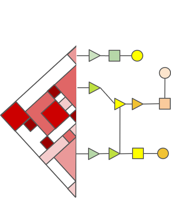

Signals pertaining to transcriptional activation are transferred from enhancers found in intergenic loci to genes in the form of transcription factors, cofactors, and various transcriptional machineries such as RNA Pol II. How and where this information is transmitted to and from is central for decoding the regulatory landscape of any gene and identifying enhancers. Esearch3D is an unsupervised algorithm to predict enhancers. It reverses engineering the flow of information and identifies intergenic regulatory enhancers using solely gene expression and 3D genomic data. It models chromosome conformation capture (3C) data as chromatin interaction network (CIN) and then exploits graph-theory algorithms to integrate RNA-seq data to calculate an imputed activity score (IAS) for intergenic regions. We also provide a visualisation tool to allow an easy interpretation of the results.

Features

1. It uses the expression levels of genes and a chromatin interaction network to impute the activity score of enhancers represented as nodes
2. It reverse engineers the flow of information modeled by enhancers that act as regulatory sources to increase the rate of transcription of their target genes
3. It leverages the relationship between the 3D organisation of chromatin and global gene expression
4. It represents a novel enhancer associated feature that can be used to predict enhancers
5. It provides a graphical user interface to interact with the network composed by genes, enhancers and intergenic loci associated to thier imputed activity score
6. It includes a parallelized version of the network-based algorithm called random walk with restart that works on sparce matrices to reduce the system usage

Citation

Manindeer *, Giudice * et al. Esearch3D: Propagating gene expression in chromatin networks to illuminate active enhancers

*equally contributed

Install

Esearch3D is available on R, you can install it by:

install.packages("devtools")
install.packages("htmltools", version="0.5.2", type="source")
devtools::install_github(
  repo="LucaGiudice/Esearch3D",
  ref = "main",
  dependencies = "Depends",
  upgrade = "always",
  quiet = T
  # type = "binary" # usable only in Windows OS
)

Vignettes

There are the following vignettes:

1. Quick Start with Dummy data
2. Vignette with TSS data without enhancer annotation
3. Vignette with WG data without enhancer annotation
4. Vignette with WG bait data with enhancer annotation and Machine Learning
5. Vignette with WG other end data with enhancer annotation and Machine Learning

Representation of chromatin data

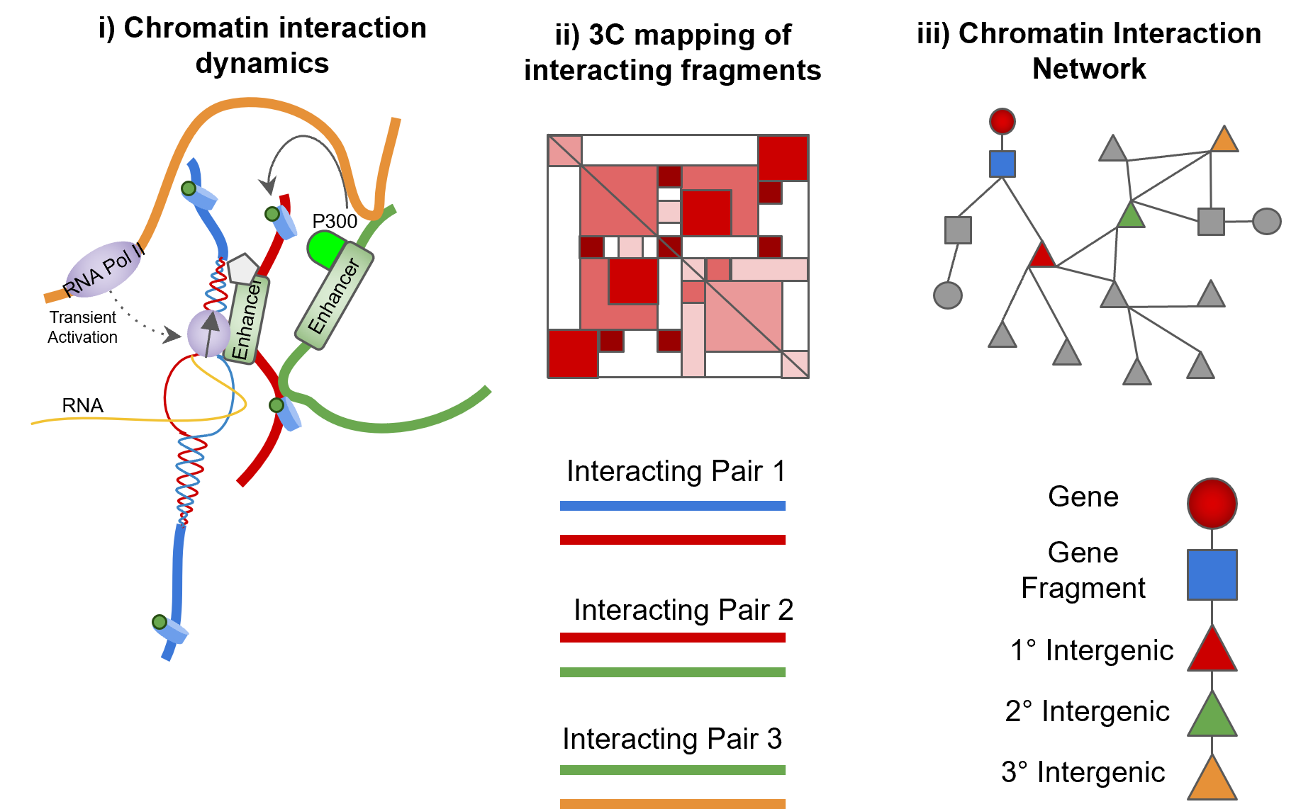
Schematic of converting chromatin dynamics into networks:

1. Enhancers are localised and can influence the regulation of promoters directly and indirectly.
2. 3C can capture chromatin interactions but only in a pairwise manner.
3. Representation of chromatin fragments as nodes in a network and their interactions as edges preserves indirect associations between interacting chromatin.

Representation of two step propagation

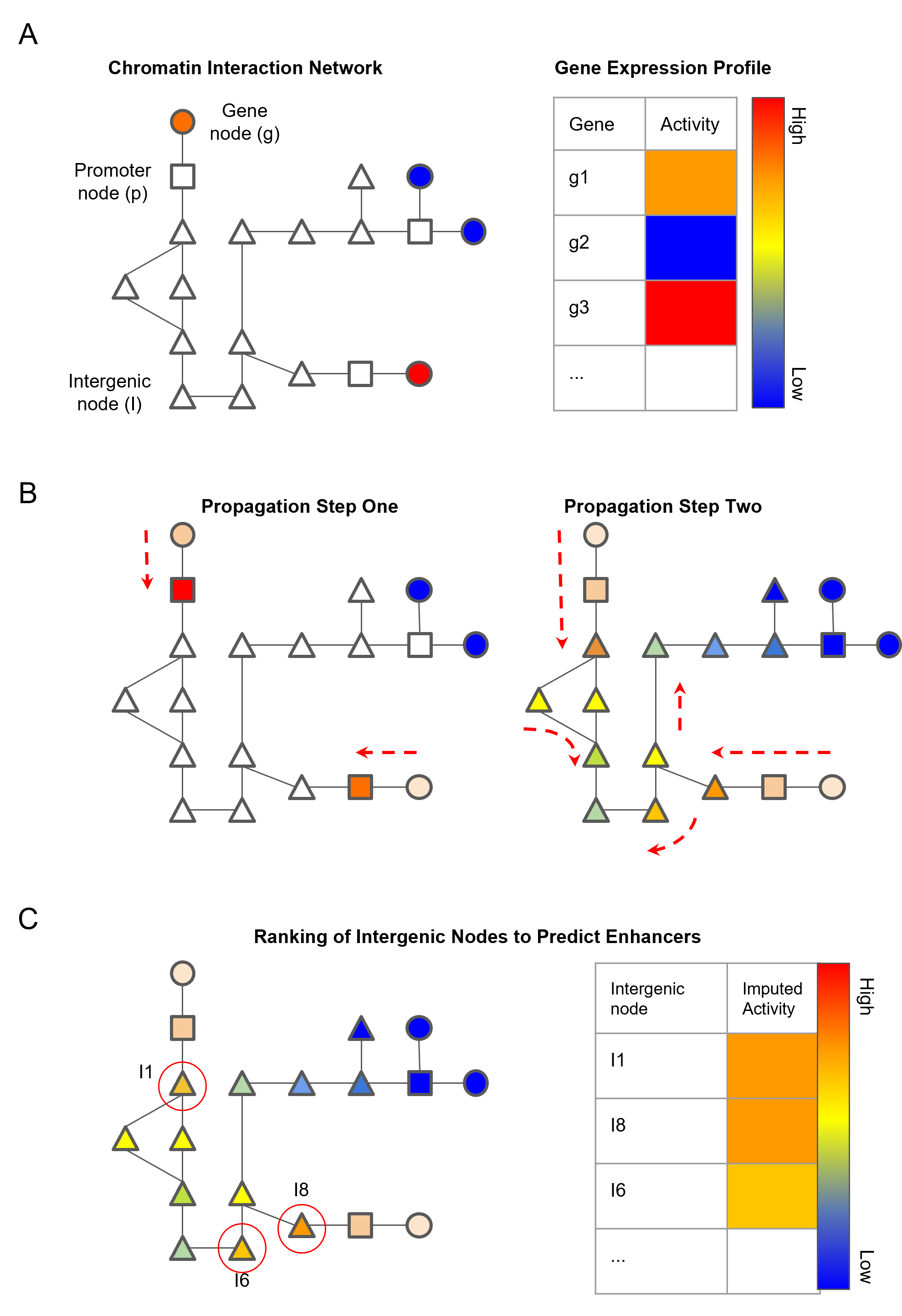
Schematic diagram of the network propagation used to impute activity values at intergenic nodes:

• A. Genes are mapped to nodes representing genic chromatin fragments. Each gene has an associated gene activity value determined by RNA-seq data.
• B. Gene activity is propagated from gene nodes to genic chromatin nodes in propagation step one. Activity scores are then imputed in intergenic chromatin nodes by propagating the scores from genic chromatin nodes.
• C. Ranking of non-genic nodes by the imputed activity score to identify high confidence enhancer nodes.

Difference from two step propagation (aka multi gene propagation) and the single gene propagation

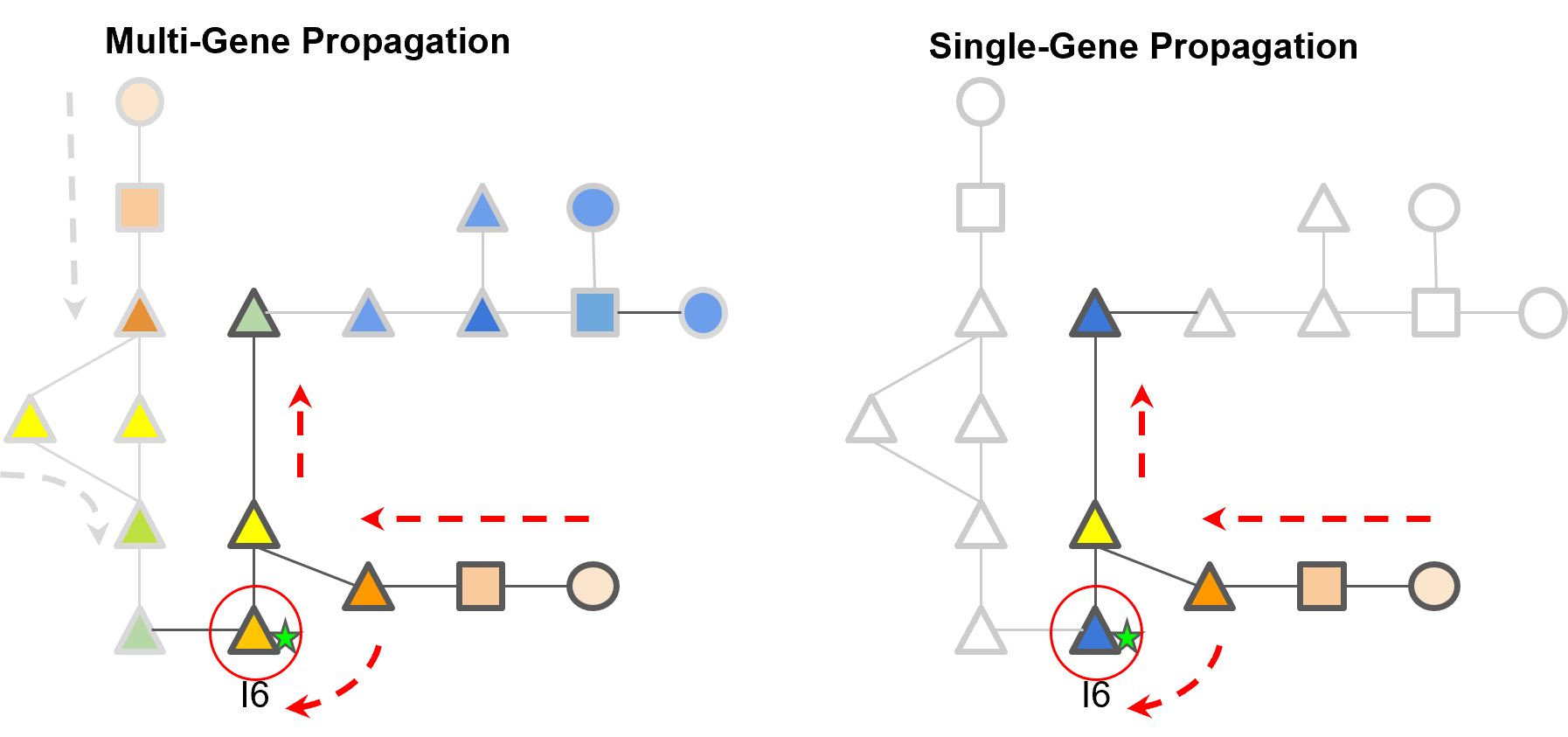
A schematic of how multi-gene and single-gene propagation differ in the relative imputed activity scores. Multi-gene propagation highlights I6, an enhancer labelled node, with a higher IAS than single-gene propagation.

Usage

Few lines of code to run D3SearchE prediction:

library(Esearch3D)

#Load and set up the example data ----
data("dummy_data_l")
#gene - fragment interaction network
gf_net=dummy_data_l$gf_net
#gene-fragment-fragment interaction network
ff_net=dummy_data_l$ff_net
#sample profile with starting values for genes and fragments
input_m=dummy_data_l$input_m
#length of chromosomes
chr_len=dummy_data_l$chr_len
#gene annotation
ann_net_b=dummy_data_l$ann_net_b

#Two step propagation -----
#Propagation over the gene-fragment network
gf_prop=rwr_OVprop(g=gf_net,input_m = input_m, no_cores=2, r=0.1)
#Propagation over the gene-fragment-fragment network
ff_prop=rwr_OVprop(g=ff_net,input_m = gf_prop, no_cores=2, r=0.8)

#Create igraph object with all the information included
net=create_net2plot(gf_net,input_m,gf_prop,ann_net_b,frag_pattern="F",ff_net,ff_prop)

#Start GUI
start_GUI(net, ann_net_b, chr_len, example=T)

#Single gene propagation -----
degree = 3
frag_pattern = "F"
gene_in=c("G1")

contrXgene_l=rwr_SGprop(gf_net, ff_net, gene_in, frag_pattern,
                        degree = degree, r1 = 0.1, r2 = 0.8, no_cores = 2)

#Create igraph object with all the information included
sff_prop=as.matrix(contrXgene_l$G1$contr_lxDest$ff_prop[,gene_in])
colnames(sff_prop)=gene_in
#Create igraph object with all the information included
net=create_net2plot(gf_net,input_m,gf_prop,ann_net_b,frag_pattern="F",ff_net,ff_prop)

#Start GUI
start_GUI(net, ann_net_b, chr_len, example=T)

GUI

1. It allows to explore a sample's profile after a network-based propagation
2. It allows to investigate the imputed activity scores obtained by specific genes and their neighbourhood
3. It allows to download the propagated network and to import it in cytoscape

Legend

1. Select nodes by chromosomes: allows to filter the network and to keep only those nodes (e.g. genes) that belong to a specific chromosome
2. Select nodes by genome region: allows to filter the network and to keep only those nodes that belong to a specific genome region
3. Select or type node + Distance: allows to visualize the neighbourhood of one specific node of interest
4. Select by propagation ranges: allows to filter the subnetwork generated with a "search". It allows to keep only the nodes with a value that falls inside a specific range
5. Scale colours: allows to scale the colors of the visualized nodes as if the propagation would have been applied only on them
6. More/Less: allow to increase or decrease the size of the neighbourhood around a node of interest based on the distance (e.g. first degree neighbourhood, second degree ...)
7. Open in cytoscape: allows to open the network in cytoscape
8. Download: allows to download the image of the network visualized and created with the GUI

Plots

Following plot shows you an example of how to interact with the GUI and its functionalities

License

MIT @ Giudice Luca

LucaGiudice/Esearch3D documentation built on Dec. 17, 2021, 1:12 a.m.